Vision Transfomer
(Dosovitskiy et al., 2020)
MLP-Mixer
SwinTransformer
Swin Transformer architecture is proposed to build feature maps hierarchically at each stage. It does this by starting from small-sized patches (patches are same as in original ViT) and gradually merging neighbouring patches in each successive layers. It helps computing self-attention locally within non-overlapping window, and as each window size is fixed, computational complexity becomes linear to image size.
However, the key design change is Shifting Windows that bridges the windows of successive layers. In any layer $l$, a certain window partitioning scheme is adopted and self-attention is computed at it. With Shifting windows, at next layer of $l+1$, window partitioning is shifted by $M/2$ (More on $M$ later) which results in new windows and the self-attention computation would now cross the boundaries of the previous windows, thus providing connection among them. (Liu et al., 2021)
Swin Transformer Architecture
At the beginning, like ViT, we first split the RGB image into non-overlapping patches and each patch is treated as a token.
We use a patch size of $4 \times 4$, and thus feature dimension of each patch is $4 \times 4 \times 3 = 48$.
So, if we have image of height and width $H \times W$, we get $\frac{H}{4} \times \frac{W}{4}$ tokens, each with 48 dimensions
Stage 1 : After this preliminary work, we enter into stage 1, where first a linear embedding layer is applied on this raw-valued feature to map it into dimension $C$. Then, several Swin Transformer blocks are applied, while maintaining output of $\frac{H}{4} \times \frac{W}{4} \times C$ size.
Also, value of $C$ is the design choice
Stage 2 :
Patch Merging As networks starts to get deeper with each successive stage, a concept of Patch Merning is introduced. Here, we concatenate $2 \times 2$ neighbouring patches, and since each patch has $C$ dimension vector, after concatenation, we get $4C$-dimensional feature vector.
Next, we apply a linear layer where output dimension is set to $2C$. Afterwards, again Swin Transformer blocks are applied where output size is now $\frac{H}{8} \times \frac{W}{8} \times 2C$
Stage 3 : Similar combination of Patch Merging and Swin Transformer is applied again with changed output size of $\frac{H}{16} \times \frac{W}{16} \times 4C$
Stage 4 : Another pair of Patch Merging + Swin Transformer block with further change in output as $\frac{H}{32} \times \frac{W}{32} \times 8C$.
This is evident in the image below (taken from source research paper)
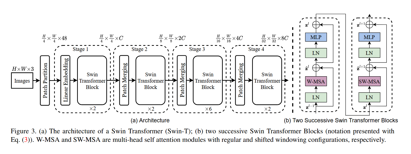
Swin Transformer Block
As in the image above, Swin Transformer block consists of two transformers where output from one is pushed into another. First transformer is Window-Multi Head Self-Attention (W-MSA), and Shifted-Window-MSA, (SW-MSA) later.
In the block, first we have LayerNorm (LN), (it is applied before each MSA or MLP module) then W-MSA or SW-MSA, which is followed by residual connection, (residual connection is after each MSA or MLP module)
Let $z^{l-1}$ be input tp block $l$,
then regular block with W-MSA is as:
\(\hat{z}^l = \text{W-MSA}(\text{LN}(z^{l-1})) + z^{l-1}\) \(z^{l} = \text{MLP}(\text{LN}(\hat{z}^l)) + \hat{z}^l\)
and, the next SW-MSA computation is as:
\(\hat{z}^{l+1} = \text{SW-MSA}(\text{LN}(z^{l})) + z^{l}\) \(z^{l+1} = \text{MLP}(\text{LN}(\hat{z}^{l+1})) + \hat{z}^{l+1}\)
Efficient Batch Computation for SW-MSA
In the Shifted configuration, we get more windows than earlier with few smaller than original $M \times M$, and total number of windows increase from $[\frac{h}{M}] \times [\frac{w}{M}]$ to $\left([\frac{h}{M}] +1\right) \times \left([\frac{w}{M}] +1\right)$.
$M$ is the design choice usually 7, and we shift window by $M/2$. To avoid inefficiency due to varied sizes of windows, we use cyclic shift towards top-left, moving up by 2 rows, and left by 2 columns. After this, we employ regular window partitioning and compute self-attention.
However, now that we have tokens from different section of images next to each other, which shouldn’t get mixed. We use masking mechanism . In any windows, if tokens were from the original image region, we allow attention, otherwise not
Lastly, we reverse the cyclic shift, to get back original for next W-MSA.
DeiT
Data Efficient Image Transformer (DeiT) architecture is almost equivalent to original ViT. However, it has an additional distillation token added alongside class token and patch token before being passed into self-attention (Touvron et al.,2021).
Distillation token is output by the network after final layer, and its target objective is given by the distillation component of the loss.
Other Changes:
- A Feed-Forward Network (FFN) is added on top of MSA layer. This FFN is composed of two linear layers separated by GeLU
- MLP Head is not used for pre-training, but only a linear classifier
Distillation :
It refers to the knowledge transferring paradigm during training from a teacher model to student. A student model leverages “soft” labels coming from a strong teacher model.
It can be of two types:
Soft Distillation : Soft Distillation minimises the Kullback-Leibler divergence between the softmax of the teacher and the softmax of the student model.
If $Z_t$ be the logits of teacher model, $Z_s$ the logits of the student model, and $\tau$ denote the temperature for the distillation, and $\lambda$ the coefficient balancing KL Divergence and the cross-entropy on ground truth labels $y$ and $\psi$ the softmax function. The distillation objective is:
$L_{\text{global}} = (1 - \lambda) L_{\text{CE}}(\psi(Z_s),y) + \lambda \tau^2 \text{KL}(\psi(Z_s / \tau), \psi(Z_t /\tau))$
Hard Distillation : Hard distillation is when hard label of the teacher is taken as true label by student. Let $y_t = \text{argmax}_c Z_t(c)$ be the hard decision of the teacher, the objective can be stated as:
\[L_{\text{hard dist. Globl}} = \frac{1}{2} L_{\text{CE}}(\psi(Z_s), y) + \frac{1}{2} L_{\text{CE}}(\psi(Z_s), y_t)\]T2TViT
Tokens-to-Token Vision Transformer (T2T-ViT) is proposed to resolve two limitations of ViT
- Standard tokenisation procedure makes ViT unable to capture local image structures such as edges, and lines efficiently, thus requiring more training samples
- Backbone of ViT is not well-designed leading to limited feature richness
Also, ideally T2T-ViT is expected to perform better than DeiT (Yuan et al., 2021)
T2T-ViT Architecture
T2T-ViT has two main components
-
T2T-ViT Module : It progressively structurizes the image with a layer-wise “Tokens-to-token module” to model to local structure information and reduce token length iteratively. It has two steps:
-
Restructurization : In this, the sequence of token $T$ coming from preceding transformer layer is transformed by self-attention block as: \(T^{'} = \text{MLP}(\text{MSA}(T))\)
Next, obtained tokens $T^{‘}$ gets reshaped into an image, i.e, $I = \text{Reshape}(T^{‘})$.
Here $\text{Reshape}$ re-organizes token $T^{‘} \in \mathbb{R}^{l \times c}$ to $I \in \mathbb{R}^{h \times w \times c}$, where $l$ is the length of $T^{‘}$ and $l = h \times w$, and $h, w, c$ are height, width and channel, respectively as in the image below:
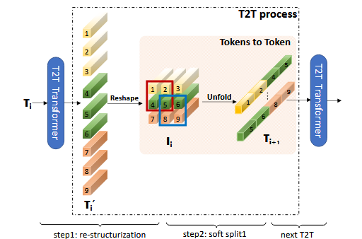
- Soft Splits : In this, we split restructurized image from the previous step into patches with overlapping. Key: as in the image above - tokens in each split patch are concatenated as one token (Tokens-to-Token). This helps aggregating local information from pixels and patches while reducing tokens.
Size of each patch is $k \times k$ with $s$ overlapping and $p$ padding on the image, where $k-s$ is similar to the stride in convolution operation.
So, the length of output token $T_{out}$ after soft split from reconstructed image $I$ can be written as:
\[l_{out} = \left[ \frac{h + 2p - k}{k - s} + 1\right] \times \left[ \frac{w + 2p - k}{k - s} + 1\right]\]Output tokens are then fed into the next T2T process. However, we start with input image $I_{0}$, so we first apply Soft Split to get our first set of tokens $T_{0}$, before starting T2T-ViT Module as: \(T_{0} = \text{SS}(I_0)\) \(T_{0}^{'} = \text{MLP}(\text{MSA}(T_0))\) \(I_1 = \text{Reshape}(T_{0}^{'})\) \(T_{1} = \text{SS}(I_1)\)
Key thing is as the length of tokens in the T2T module is larger than the normal case, the MAC and memory usage are huge, therefore, channel dimension of T2T-Vit module is set to 32 or 64.
-
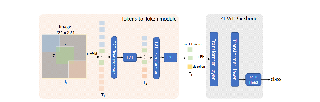
T2T-ViT Backbone : To draw global attention relation on tokens from T2T module, T2T-ViT uses deep narrow architecture for backbone. Here, deep means increased layer depth which improves feature richness in ViT, and narrow means decreased channel dimension to reduce the redundanct in channels.
- T2T-ViT backbone has small channel and a hidden dimension $d$ but more layers $b$
- For tokens with fixed length $T_f$ from the last layer of T2T module, a class token and Sinusoidal Position Encoding (PE) is added before pushing it into ViT for classification as:
Complete architecture is best illustrated in the main paper as below:
ConViT
Self-Attention(SA) have no built-in understanding of image structure, and learns it from scratch (low inductive bias), whereas CNNs have strong spatial locality imbued in them (strong inductive bias). To balance between both of them, ConViT, idea, is to let each SA layer decide whether to behave like a convolutional layer or SA layer by introducing Gated Positional Self-Attention (GPSA) (d’Ascoli et al., 2021).
GPSA is evolved over Positional Self-Attention (PSA). Cordonnier et al. (2019) showed that multi-head PSA layer with $N_h$ heads can perfectly mimic convolutional layer of size $\sqrt{N_h} \times \sqrt{N_h}$.
We know that, standard PSA is expressed as:
\[A_{ij}^h := \text{Softmax}(Q_{i}^h (K_{j}^h)^T + (v_{\text{pos}}^h)^T r_{ij})\]where $v_{\text{pos}}$ is the trainable embedding that acts as an “attention center” determining which relative distance head should focus on. $r_{ij}$ is relative positional embedding - the distance between the pixel $i$ and $j$. However, to use Transformer as a Convolution, we need to use following settings:
- $W_{\text{query}} = W_{\text{key}} = 0$ - to turn off content-similarity, and focus on where the pixel is, than what the pixel is.
- $W_{key} = I$ - Output is direct unmodified copy of input’s feature weighted by attention score.
- $r_{\delta}$ - A fixed 3-dim vector for physical distance between query patch $i$ and key patch $j$.
- Dim 1 - $\lVert \delta \rVert^2$ - the squared total distance
- Dim 2 - $\delta_1 $ - the horizontal x-axis distance
- Dim 3 - $\delta_2 $ - the vertical y-axis distance
- $v_{\text{pos}^h} := -\alpha^h(1, -2\Delta_1^h, - 2\Delta_2^h)$
Thus, $(v_{\text{pos}}^h)^T \cdot r_{\delta} = -\alpha^h \left( 1 \cdot \lVert \delta \rVert^2 + (-2\Delta_1^h)\cdot \delta_1 +(-2\Delta_2^h)\cdot \delta_2 \right)$
$\implies (v_{\text{pos}}^h)^T \cdot r_{\delta} = -\alpha^h \left( \lVert \delta \rVert^2 -2\Delta_1^h \delta_1 -2\Delta_2^h \delta_2 \right)$
$\implies (v_{\text{pos}}^h)^T \cdot r_{\delta} = -\alpha^h \lVert \delta - \Delta^h \rVert^2 + \text{C}$
As the value of constant $\text{C}$ would be nagated by softmax, the attention score would become directly proportional to it as: $A_{ij} \propto \text{exp}\left(-\alpha^h \lVert \delta - \Delta^h \rVert^2\right)$, making it resemble Gaussian curve. Therefore,
- The center of attention $\Delta^h \in \mathbb{R}^2$ will get the most attention by the head $h$.
- The locality strength $\alpha^h \gt 0$ or _temperature of softmax will determine how focussed is attention towards its center $\Delta^h$
- If $\alpha^h$ is large, head is focussed on exact pixels/patches at $\Delta^h$ making it behave like Convolution layer.
- If $\alpha^h$ is small, the attention of head is spreadout onto a larger area of patches
Positional Self Attention (PSA) however, have two backdrops:
- Vast number of trainable parameter for $r_{\delta}$ is quadratic. This is solved by keeping the $r_{\delta}$ fixed, and training only the $v_{\text{pos}}^h$ which determines the center and span of attention
- Convolutional initialization before the softmax makes it blind With convolutional intialization we start to get positional term $(v_{pos}^h)$ highly concentrated. This results in very high positional score and very low content score, and the smallest of both - content score thus gets ignored by the softmax making it blind convolution. This provides greater boost in earlier phase of training but lazily ignores the content score when training progresses.
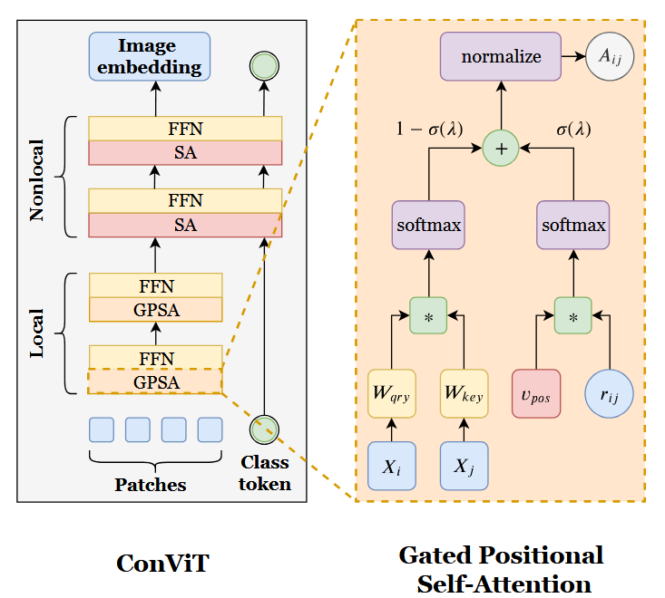
Gated Positional Self Attention (GPSA):
GPSA solves this problem of PSA by adding the content and positional term after the softmax, with their relative importance governed by the learnable Gating Paramter ($\lambda$). We can write resulting GPSA parametrized as:
\[\text{GPSA}_h (X) := \text{normalize} [A^h] XW_{\text{val}}^h\] \[A_{ij}^h := (1-\sigma (\lambda_h)) \text{softmax} (Q_{i}^h (K_{j}^h)^T) + \sigma(\lambda_h)\text{softmax}((v_{\text{pos}}^h)^T \cdot r_{ij})\]Here, adding the content and positional term after the softmax makes sure both values are normalized to sum to 1. Gating Parameter ($\lambda_h$) acts as mixing board which with sigmoid acts a gate for pure transformer and convolution as :
- If $\lambda$ is very negative, $\sigma(\lambda_h) \approx 0$ making layer pure content - transformer
- If $\lambda$ is very positive, $\sigma(\lambda_h) \approx 1$ making layer pure position - convolution
However, paper used the value of $\lambda_h$ as $1$. This makes $\sigma(1) = 0.73$ i.e, 73% positional and 27% content. With increasing number of epochs as $\lambda_h$ would start to get smaller, attention score for content will start to increase.
ConvMixer
ConvMixer is, essentially, exploring the question of whether the strong performance of vision transformers is resulted more from patch-based representation than Transformer. For this reason, transformer is not used, but standard convolution.
In ConvMixer, after patch embedding, there is no downsampling of the representation at successive layers, thus maintaining equal-resolution-and-size throughout. Additionally, it separates channel-wise-mixing and spatial-wise-mixing, by choosing depthwise convolution for mixing spatial locations, and pointwise convolution for mixing channel locations (Trockman and Kolter, 2022).
ConvMixer Architecture:
Patch Embedding:
If we have input image as $X \in \mathbb{R}^{C_{in}\times H \times W}$ and patch size $p$, and embedding dimension $h$, then patch embedding can be done with standard convolution with $C_{in}$ as input channels, and $h$ as output channel and patch size $p$ to be used as kernel and stride as :
\[z_{0} = \text{BN}(\sigma \{\text{Conv}_{in \rightarrow h} (X, \text{stride}=p, \text{kernel_size}=p)\})\]where $\sigma$ is activation function of GELU, and $\text{BN}$ is Batch Normalization. After embedding, spatial dimensions are reduced by $p$, and $h$ becomes channel dimension, expressed as $z_{0} = \mathbb{R}^{h\times \frac{H}{p} \times \frac{W}{p}}$

ConvMixer Layer:
It has two main component into it - Depthwise convolution for spatial location mixing and Pointwise convolution for channel wise mixing. Both are followed by activation function (GELU) and Batch Normalization. Afterwards, we repeat this combination $d$ times.
In Depthwise, we set groups=h, so that channels never mix, and we get separate convolution per channel, and set kernel_size $k$ to be a large number (7 or 8). In addition, residual connection is used which adds input of depthwise convolution to the output after BathNorm.
In Pointwise, there is no residual connection. Also, we pick kernel_size to be $1 \times 1$, input and output channels are set at $h$. We can illustrate both process of ConvMixer layer as:
Global Pooling and Classification :
After $d$ repeat of ConvMixer block, we get final output as $z_{d} = \mathbb{R}^{h \times \frac{H}{p} \times \frac{W}{p}}$ on which we perform global pooling to get a feature vector of size $h$. Output of this then passed into softmax for final classification
\(\text{FeatureVec} = \text{GlobalAvgPool}(z_{d}) \in \mathbb{R}^h\) \(\hat{y} = \text{Softmax}(W \cdot \text{FeatureVec} + b)\)
where, $W \in \mathbb{R}^{C_{out}\times h}, C_{out}$ = number of classes
MaxViT
(Tu et al., 2022)
References
- d’Ascoli, S., Touvron, H., Leavitt, M.L., Morcos, A.S., Biroli, G. and Sagun, L., 2021, July. Convit: Improving vision transformers with soft convolutional inductive biases. In International conference on machine learning (pp. 2286-2296). PMLR.
- Dosovitskiy, A., Beyer, L., Kolesnikov, A., Weissenborn, D., Zhai, X., Unterthiner, T., Dehghani, M., Minderer, M., Heigold, G., Gelly, S. and Uszkoreit, J., 2020. An image is worth 16x16 words: Transformers for image recognition at scale. arXiv preprint arXiv:2010.11929.
- Trockman, A. and Kolter, J.Z., 2022. Patches are all you need?. arXiv preprint arXiv:2201.09792.
- Touvron, H., Cord, M., Douze, M., Massa, F., Sablayrolles, A. and Jégou, H., 2021, July. Training data-efficient image transformers & distillation through attention. In International conference on machine learning (pp. 10347-10357). PMLR.
- Tu, Z., Talebi, H., Zhang, H., Yang, F., Milanfar, P., Bovik, A. and Li, Y., 2022, October. Maxvit: Multi-axis vision transformer. In European conference on computer vision (pp. 459-479). Cham: Springer Nature Switzerland.
- Liu, Z., Lin, Y., Cao, Y., Hu, H., Wei, Y., Zhang, Z., Lin, S. and Guo, B., 2021. Swin transformer: Hierarchical vision transformer using shifted windows. In Proceedings of the IEEE/CVF international conference on computer vision (pp. 10012-10022).
- Yuan, L., Chen, Y., Wang, T., Yu, W., Shi, Y., Jiang, Z.H., Tay, F.E., Feng, J. and Yan, S., 2021. Tokens-to-token vit: Training vision transformers from scratch on imagenet. In Proceedings of the IEEE/CVF international conference on computer vision (pp. 558-567).