Augmentation
Random Erasing
Random Erasing (RE) is another method that does not require additional memory consumption, and parameter-free. In RE, a rectangular region $I_e$ is randomly selected, and its pixels are erased and replaced with random values . This can be considered as adding noise to the image while preserving overall image structure, to make the learning more robust.
In this method, for an image $I$ in mini-batch, the probability of it being selected for RE is at $p$, and kept unchanged is $1-p$ in this transformation.
Now, lets assume if the size of training image $I$ selected with $p$ probability is $W \times H$, then area would be $S = W \times H$.
So, we randomly initialize area of rectangular region for erasing as $S_e$, where $\frac{S_e}{S}$ is in range of minimum $(s_l)$ to max $s_h$, and aspect ratio of rectangle between $r_1$ and $r_2$ as $r_e$, then $H_e = \sqrt{S_e \times r_e}$ and $W_e = \sqrt{\frac{S_e}{r_e}}$.
Next, we randomly initialize a point $\mathcal{P} = (x_e, y_e)$ in $I$. If $x_e + W_e \le W$ and $y_e + H_e \le H$, we set the region, $I_e = (x_e, y_e, x+e + W_e, y_e + H_e)$ as the selected rectangle region.
- Zhong et al., (2020) used $p = 0.5$, $s_l = 0.02$, $s_h=0.4$, and $r_1 = \frac{1}{r_2} = 0.3$
CutOut
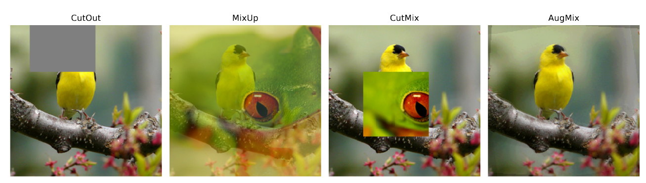
CutOut uses same random occlusion technique as RE above. Similarly, it is parameter-free, and computationally efficient. Also, again for an image $I$ in mini-batch, probability of it being selected for transformation is $p$, and remain unchanged at $1-p$, where $p =0.5$ is used in paper.
Key difference to RE is CutOut uses 1. square region to erase 2. It does not restric occlusion patch to be restriced within the image i.e, only a portion of square can be on image, rest outside.
MixUp
If we have two examples $(x_i, y_i)$ and $(x_j, y_j)$ in our dataset, where $x_i$, $x_j$ are raw input vectors (images) and $y_i$, $y_j$ are one-hot encoded label, then MixUp proposes to generate new training example $(\hat{x}, \hat{y})$ based on generic vicinal distribution as:
\[\mu (\hat{x}, \hat{y} | x_i, y_i) = \frac{1}{n} \sum_{j}^n \mathbb{E}_{\lambda} \left[\delta(\hat{x} = \lambda \cdot x_{i} + (1 - \lambda)\cdot x_j, \hat{y} = \lambda\cdot y_i + (1-\lambda)\cdot y_j) \right]\]where, $\lambda \sim \text{Beta}(\alpha, \alpha)$ for $\alpha \in (0, \infty)$
In summary, MixUp produces newer data input $\hat{x}$ and target label, $\hat{y}$ as:
\(\hat{x} = \lambda x_{i} + (1 - \lambda) x_j\) \(\hat{y} = \lambda y_{i} + (1 - \lambda) y_j\)
Here, $\alpha$ controls the stregth of interpolation between image-label pairs, recovering original if $\alpha \rightarrow 0$
CutMix
CutMix is evolved over MixUp, and can be used for all three task of classification, localization and object detection. On the other hand, MixUp results are locally ambiguous and appear unnatural, thereby confusing the model for localization and object task.
The goal of CutMix is to generate a new training sample $(\hat{x}, \hat{y})$ by combining again two training samples $(x_a, y_a)$ and $(y_a, y_b)$ and it can be expressed as:
\(\hat{x} = M \odot x_a + (1 - M) \odot x_b\) \(\hat{y} = \lambda y_a + (1 - \lambda) y_b\)
where, $M$ is a binary mask and $\odot$ is elementwise multiplication. If the mask $M$ is $1$, the new image keeps the pixels from $x_a$, if $M=0$, then new image takes pixels from $x_b$
$\lambda$ is sampled from $\text{Beta}(\alpha, \alpha)$ where default value for $\alpha =1$, making it uniform distribution $(0, 1)$.
Next, to create binary mask $M$, the method defines a bounding box $B$ with coordiantes $(r_x, r_y, r_w, r_h)$ representing the top-left corner $(x, y)$, and the width/height $(w, h)$ of the patch to be swapped. In CutMix, a rectanguar mask $M$ is used whose aspect ratio is proportional to the original image. The box coordinates are sampled uniformly as:
\(r_x \sim \text{Unif}(0, W), \qquad r_w = W\sqrt{1-\lambda}\) \(r_y \sim \text{Unif}(0, H), \qquad r_h = H\sqrt{1-\lambda}\)
making the cropped area ratio $\frac{r_w r_h}{WH} = 1 - \lambda$
CutMix with this method replaces an image rectangular region with a patch from another image and generate more locally natural images than MixUp and be illustrated by the image below:
AutoAugment
AutoAugment automate the process of finding effective data augmentation policy for a target dataset. This learned policy can then also be transferred/used with a newer dataset.
It has two components: Search Space and Search Algorithm
-
In Search Space, each policy consists of 5 sub-policies, and each sub-policies consists of two image operations.
-
We have 16 operations in our search space i.e, Shear X/Y, Translate X/Y, Rotate, AutoContrast, Invert, Equalize, Solarize, Posterize, Contrast, Color, Brightness, Sharpness, Cutout, and Sample pairing
-
Additionally, each operation has two hyperparameters (1) the probability of applying the operation, and (2) the magnitude of the operation.
-
In Search Algorithm, we have two components again i.e, a controller and a training algorithm PPO reinforcement learning method. At each step, controller provides 30 softmax predictions to predict 5 sub-policies, with 2 operations each, and each operation requiring - type, probability, and magnitude
RandAugment
RandAugment does not require a search space, thus simpler to train, and computationally cheap, in comparison of AutoAugment it is reduced from $10^{32}$ to $10^2$.
This is done by replacing the learning policy with random selection with uniform probability, if we have $K$ transformation, each transformation will have equal probability of $\frac{1}{K}$ of being picked up.
Transformations $(K=14)$ used in RandAugment are identity, rotate, posterize, sharpness, Translate X/Y, Shear X/Y, AutoContrast, Equalize, Solarize, Color, Contrast, Brightness. If a sequence of $N$ transformation is applied to a training image, RandAugment can generate $K^N$ distinct policies. Making it effective despite being “paramter-free” and much simpler.
Next, for the magnitude of each transformation, a universal integer scale from $0$ to $10$ is adopted, and instead of optimizing separate magnitude between 0 and 10 for each transformation, a single global parameter, $M$ utilized for all transformation operation
AugMix
AugMix at first, creates a chain of transformation operation, which afterwards gets combined together. Transformation operations are borrowed from AutoAugment, however those in ImageNet corruption i.e., color, contrast, sharpness,brightness, CutOut are removed.
Next, for the original image $x_{orig}$, we randomly sample $k$ augmentation chains (default $k=3$), where each chain is composed of $m$ operations, with $m$ being sampled from uniformly from ${1, 2, 3}$.
After AugMix mixes all three chains together into a single one in two stages using convex combinations.
- The $k$ transformed images $(x_1, x_2, x_3)$ for $k=3$ are combined using element-wise convex combinations. We sample a weight vector $w$ from a symmetric Dirichlet distribution.
$w \sim \text{Dirichlet}(\alpha,\cdots, \alpha)$ such that $\sum_{i=1}^k w_i = 1$ and $w_i \ge 0$. The mixed image from the chains is thus, $x_{aug} = \sum_{i=1}^k w_i x_i$
- Next, we use skip connection to combine the augmented $x_{aug}$ with the original $x_{orig}$. We sample a mixing coefficient $v$ from a Beta distribution, $v \sim \text{Beta}(\alpha, \alpha)$.
The final AugMix image, therefore, is given in the equation and image below:
\[x_{\text{augmix}} = v \cdot x_{\text{orig}} + (1-v)\cdot x_{\text{aug}}\]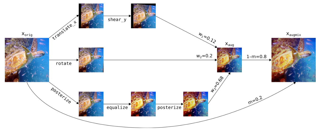
Jensen-Shannon Divergence Consistency Loss: Since the semantic content of the image $x_{orig}$ is preserved with AugMix method, we would want the model to embed original $x_{orig}$, and its two variants $x_{augmix1}$ and $x_{augmix2}$ similarly, so that output would not fluctuate wildly.
For this, we need to minimize Jensen-Shannon Divergence among the posterior distributions of the original samples and its both variants. If the posterior distribution is as:
$p_{\text{orig}} = \hat{p}(y \mid x_{\text{orig}})$
$p_{\text{augmix1}} = \hat{p}(y \mid x_{\text{augmix1}})$
$p_{\text{augmix2}} = \hat{p}(y \mid x_{\text{augmix2}})$
then, the $M$, the mixture distibution where we compute average of theses three can be expressed as:
$M = \frac{1}{3}(p_{orig} + p_{\text{augmix1}} + p_{\text{augmix2}})$
$M$ is calculate so that, KL Divergence will not reach infinity, if denominator approaches $0$. With $M$ which is the average of three - $x_{orig}, x_{augmix1}, x_{augmix2}$, KL will never explode to infinity, as the denominator will never be near zero, and that’s why two augmentation is taken, and not just one.
So, we can write now JS Divergence as:
\[JS(p_{\text{orig}};p_{\text{augmix1}};p_{\text{augmix2}}) = \frac{1}{3}\left(\text{KL}[p_{orig} || M] + \text{KL}[p_{\text{augmix1}} || M] + \text{KL}[p_{\text{augmix2}} || M] \right)\]Finally, during training, the standard cross-entropy loss is augmentted with the JS consistency loss. For an original image $x_{\text{orig}}$ with true label $y$, the total loss $\mathcal{L}_{\text{total}}$ is:
\[\mathcal{L}_{\text{total}} = \mathcal{L}_{\text{CE}}(p_{\text{orig}},y) + \lambda \cdot \text{JS}(p_{\text{orig}}, p_{\text{augmix1}}, p_{\text{augmix2}})\]Regularizations
Weight Decay
Weight Decay is another term for L2 Regularization. It is motivated by the intuition that simplest possible function would be the one where all weights are zero, i.e $f(x) = 0$. This way we can measure complexity of any function by calculating how far its parameter are from $0$. In standard training, we are minimizing a loss function $\mathcal{L}(\theta, x, y)$ where $\theta$ is the weight term. So, by adding $L2$ norm as a penalty to this loss function, we can force model to balance between training loss, and smaller $\theta$ value.
Thus, L2 Regularization can be expressed as :
\[{\tilde L(\theta)} = L(\theta) + \frac{\lambda}{2} \lVert w \rVert_2^{2}\]here, $w$ is weight vector, $\lambda$ is the weight decay coefficient $(0\gt \gt 1)$, and $\lVert w \rVert_2^{2}$ is the squared L2 norm.
While taking derivative of prior equation, $\frac{1}{2}$ gets cancelled out, and we get:
\[\frac{\partial{\tilde{L}}}{\partial w} = \frac{\partial L}{\partial w} + \lambda w\]We know that the weight update rule with a learning rate of $\eta$ is as:
\[w_{t+1} = w_t - \eta \frac{\partial \tilde{L}}{\partial w_t}\]Thus, we can expand it as using earlier eq(7) as:
\[w_{t+1} = w_t - \eta \left(\frac{\partial \tilde{L}}{\partial w_t} + \lambda w_t \right)\] \[w_{t+1} = (1 - \eta \lambda)w_t - \eta \frac{\partial L}{\partial w_t}\]This weight update rule shows that even before applying the gradients, weight shrinks by the factor of $(1 - \eta \lambda)$. That is why Weight Decay.
Dropout
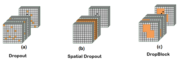
Dropout is a stochastic regularization method which randomly sets activation of hidden units to zero during training to prevent overfitting. It is, however, not suitable to be implemented in CNNs.
In a standard NeuralNet, with $L$ hidden layers, for any layer $l \in {0, 1, \cdots L-1}$, the forward pass computes the pre-activation $z^(l+1)$ and output $y$, if $W$, and $b$ are weight and biases, as:
\(z^{l+1} = W^{l+1}y^l + b^{l+1}\) \(y^{l+1} = f(z^{l+1})\),
Dropout is element-wise multiplication of $r$ in the input $y$ drawn from Bernoulli distribution with probability $p$ i.e, $r^{l} = \text{Bernoulli}(p)$ Thus, we can write
\(\tilde {y}^{l} = r^{l} \odot y^{l}\) \(z^{l+1} = W^{l+1}\tilde{y}^l + b^{l+1}\) \(y^{l+1} = f(z^{l+1})\)
SpatialDropout
If we apply standard Dropout to a convolutional output, we certainly can drop any individual pixel $f_{c,h,w}$ indepedently with $p$ drawn from Bernoulli, but it will not be effective as adjacent pixels $f_{c,h,w}$ and $f_{c,h,w+1}$ are strongly correlated in CNNs. Therefore, setting one to $0$ will still keep gradient flowing.
SpatialDropout, instead drops the entire spatial height and width of a specific feature map. Thus, with SpatialDropout, total number of trials also drops from $N_{features} \times H \times W$ to just $N_{features}$
DropBlock
Dropblock is another solution for implementing dropout properly in CNNs. Instead of dropping out independent random units or a whole feature map, it drops contiguous regions from a feature map of a layer. It has two main parameters block_size and $\gamma$.
We first randomly sample a mask $M: M_{i,j} \sim \text{Bernoulli}(\gamma)$. Then, assuming $M_{i,j}$ as the center point, we create a spatial square block with height and width block_size, and set all the values of pixel within $M$ as $0$.
Layer Normalization
Note: Batch Normaliztion discussed earlier
Layer Normalization is evolved over Batch Normalization for RNN and RNN based methods like Transformer(and Transformer-based method). The core prupose, however, is the same i.e, mitigating “covariate shift”. It occurs when the gradients with respect to the weights in one layer are highly dependent on the outputs of previous layer. If those outputs starts to change in a highly correlated fashion (especially after ReLu use), then training starts to become unstable. (Ba, Kiros, and Hinton, 2016). Batch Normalization addresses this by estimating mean and variance, and normalizing the summed inputs to each hidden unit across the training cases within a mini-batch.
Layer Normalization (LayerNorm), on the other hand, calculates the mean and variance over all the hidden units in the same layer as follows:
\[\mu^{l} = \frac{1}{H} \sum_{i}^H a_{i}^l \qquad \sigma^{l} \sqrt{\frac{1}{H}\sum_{i}^H(a_{i}^l - \mu^{l})^2}\]Under LayerNorm, all the hidden units in a layer will share the same terms of $\mu$ and $\sigma$. This prevent the need to calculate mean, and variance for each step time in standard RNN.
Let $x^t$ be the current input, $w_{hh}$ be the recurrent hidden to hidden weight matrix, $w_{xh}$ be the bottom up input to hidden weight, and $h^{t-1}$ be the previous vector of hidden states, then in a standard RNN, the summed inputs $a^t$ are calculated as:
\[a^t = W_{hh}h^{t-1} + W_{xh}x^t\]By applying LayerNorm, We can use a single set of gain(g) and bias(b) parameters to re-center and re-scale the RNN activations across all time steps as:
\[h^t = f\left[ \frac{g}{\sigma^t} \odot (a^t - \mu^{t}) +b \right]\]Stochastic Depth
It is a regularization technique for deep network (especially with residual connections). To resolve vanishing gradient, diminishing feature re-use, and extensive training time, it is based on contrarian view of having deep network during testing, but short network for training. In a way, it can also be interpreted as having ensemble of network with different depths (Huang et al., 2016).
Therefore, stochastic depth stochastically skip layers during training and bypasses its transformation through skip connections. Let $b_l \in {0,1}$ be a $\text{Bernoulli}$ random variable indicating whether the $l^{th}$ ResBlock is active or not.
Thus, stochastic depth can bypass the $l^{th}$ Resblock by multiplying its function $f_l$ with $b_l$ and the update rule of ResBlock can be extended as:
\(H_l = \text{ReLU}\left(b_l f_l (H_{l-1}) + \text{id}(H_{l-1})\right)\).
If we would want to keep ResBlock active, we can keep $b_l=1$, and update rule remains unchanged. However, if we want to bypass ResBlock, we can make it inactive by changing to $b_l=0$, and we get (for $H_{l-1}$) is always non-negative and $\text{ReLU}$ acts as $\text{identity}$ for non-negative inputs : \(H_l = \text{id}(H_{l-1})\)
Instead of using of $\text{Bernoulli}$ variable $b_l$, we can also use a Survival Probability $(p_l)$, which linearly decay from $p_0 = 1$ for the input to $p_L$ for the last ResBlock. Since earlier layers extract low-level features, it should be present, whereas later layers can be dropped more frequently. Survival Probability $(p_l)$ thus can be expressed as:
\[p_l = 1 - \frac{l}{L}(1 - p_L)\]Here, $L$ is the total number of ResBlock, $l$ is current block, $p_l$ is survival probability of last ResBlock. Paper, though, suggested to use $p_L = 0.5$ throughout. Also, Stochastic Depth is very effective with BatchNorm.
LayerScale
LayerScale is another technique presented to improve residual architecture of deep network. It is presented for improving ViT optimization, but can be used in any residual network. Also, more of a normalization/optimization technique than regularization technique.
In general, with input $x_l$ at layer $l$, ViT can be said as network alternating between self-attention layer and FFN layer as:
\(x_l^{'} = x_l + \text{SA}(\eta(x_l))\) \(x_{l+1} = x_l^{'} + \text{FFN}(\eta(x_l^{'}))\)
LayerScale add a learnable diagonal matrix on the output of each residual block. It is a per-channel multiplication of vector produced by each ResBlock, instead of single scalar value (Touvron et al.,2021). ViT can now be expressed as:
\[x_l^{'} = x_l + \text{diag}(\lambda_l, 1, \cdots, \lambda_l,d) \times \text{SA}(\eta(x_l))\] \[x_{l+1} = x_l^{'} + \text{diag}(\lambda_l^{'}, 1, \cdots, \lambda_l^{'},d) \times \text{SA}(\eta(x_l^{'}))\]where, $\eta(\cdot)$ is Layer Normalization, $d$ is the hidden dimension or channel size, and $\lambda_{l,i}$ and $\lambda_{l,i}^i$ are learnable weights. The diagonal values are all intialized with a small fixed value of $\epsilon$, where in paper, $\epsilon = 0.1$ unit depth 18, and $\epsilon = 10^{-5}$ for depth 24, and $\epsilon = 10^{-6}$ for further deeper networks.
Label Smoothing
Standard setup for training a classifier: For a given input $x$, the model gives un-normalized scores called logits $(z_k)$ as an output for each class $k \in {1,\cdots K }$, which are then passed onyo a softmax function to get prediction on output probability distribution $p(k \lvert x)$ as $p(k \lvert x) = \frac{\text{exp}(z_k)}{\sum_i^k \text{exp}(z_i)}$.
Similarly, Ground-Truth Distribution $q(k \lvert x)$ can be expressed as dirac delta function as $q(k\lvert x) = \delta_{k,y}$, for usually it is one-hot encoded vector, where if thh true label is $y$, then $q(y) = 1$ and $q(k) = 0$ for all $k \neq y$
Afterwards, model is trained by minimizing the cross-entropy loss $l$ between the prediction $p$, and ground-truth $q$ as:
\[l = - \sum_{k=1}^K q(k) \text{log}(p(k))\]We have, $q(k)$ as one-hot encoded vector, so minimizing loss would be equal to maximizing the expect log-likelihood of the label, thus can be expressed as: $l = - \text{log}(p(y))$. Gradient of this loss with respect to the logits $z_k$ is simple: $\frac{\partial l}{\partial z_k} = p(k) - q(k)$, and bounded between $-1$ and $1$
To minimize loss function $l$, the model must push $p(y)$ as close to $1$, and for $p(y) \rightarrow 1$, we will need logit of label $z_y$ much larger than $z_k$ for all $k \neq y$.
This creates two problems:
- overfitting : model learn to assign 100% probability to the ground-truth label, where it is not guaranteed to generalize.
- As we need $p(y) \rightarrow 1$, which needs logit of label $z_y$ much larger than $z_k$ for all $k \neq y$, and having gradients bounded between -1 and 1, model become oover-confident predicting $p(y)=1$ and $p(k \neq y) = 0$, which reduces ability of model to adapt.
Label Smoothing Mechanism :
Consider a distribution over labels $u(k)$, (independent of $x$ and of uniform distribution), and a smooothing parameter $\epsilon$.
Next, we replace the label distribution $q(k) = \delta_(k,y)$ with $q^{‘} (k \lvert x)$ which is a mixture of the original ground-truth distribution $q(k \lvert x)$ and the uniform prior $u(k)$ with weights $1- \epsilon$ and $\epsilon$ as:
\[q^{'} (k \lvert x) = (1-\epsilon)\delta_{k,y} + \epsilon u(k)\]Now, with smooth distribution $q^{‘}$, we can expressed cross-entropy loss, $l$ as:
\[l = - \sum_{k=1}^K q^{'}(k) \text{log}(p(k))\] \[\implies l = -\sum_{k=1}^K \left[ \left(1-\epsilon\right) \delta_{k,y} + \epsilon u(k) \right]\text{log}(p(k))\] \[\implies l = (1 - \epsilon) \left[-\sum_{k=1}^K \delta_{k,y} \text{log}(p(k)) \right] + \epsilon \left[- \sum_{k=1}^K u(k)\text{log}(p(k)) \right]\]These two are the definitions of cross-entropy $\mathcal{H}$, thus we can simplify it as:
\[l = (1- \epsilon)\mathcal{H}(q,p) + \epsilon \mathcal{H}(u,p)\]Thus, we can say that Label Smoothing is equivalent of training model with two cross-entropy losses
- $\mathcal{H}(q,p)$ cross-entropy between prediction & ground-truth label
- $\mathcal{H}(u,p)$ cross-entropy between prediction & uniform prior
scacled by $(1-\epsilon)$ and $\epsilon$, respectively.
P.S. Use $\epsilon = 0.1$ in most cases, $0.05$ - when training on small dataset, and larger $\epsilon = 0.15 \text{or above}$ when training on massive dataset.
References
- Ba, J.L., Kiros, J.R. and Hinton, G.E., 2016. Layer normalization. arXiv preprint arXiv:1607.06450.
- Ekin D Cubuk, Barret Zoph, Jonathon Shlens, and Quoc V Le. Randaugment: Practical automated data augmentation with a reduced search space. arXiv preprint arXiv:1909.13719, 2019.
- Ekin Dogus Cubuk, Barret Zoph, Dandelion Mane, Vijay Vasudevan, and Quoc V. Le. AutoAugment: Learning augmentation policies from data. CVPR, 2018.
- Ghiasi, G., Lin, T.Y. and Le, Q.V., 2018. Dropblock: A regularization method for convolutional networks. Advances in neural information processing systems, 31.
- Huang, G., Sun, Y., Liu, Z., Sedra, D. and Weinberger, K.Q., 2016, September. Deep networks with stochastic depth. In European conference on computer vision (pp. 646-661). Cham: Springer International Publishing.
- Hendrycks, D., Mu, N., Cubuk, E.D., Zoph, B., Gilmer, J. and Lakshminarayanan, B., 2019. Augmix: A simple data processing method to improve robustness and uncertainty. arXiv preprint arXiv:1912.02781.
- Srivastava, N., Hinton, G., Krizhevsky, A., Sutskever, I. and Salakhutdinov, R., 2014. Dropout: a simple way to prevent neural networks from overfitting. The journal of machine learning research, 15(1), pp.1929-1958.
- Szegedy, C., Vanhoucke, V., Ioffe, S., Shlens, J. and Wojna, Z., 2016. Rethinking the inception architecture for computer vision. In Proceedings of the IEEE conference on computer vision and pattern recognition (pp. 2818-2826).
- Tompson, J., Goroshin, R., Jain, A., LeCun, Y. and Bregler, C., 2015. Efficient object localization using convolutional networks. In Proceedings of the IEEE conference on computer vision and pattern recognition (pp. 648-656).
- Touvron, H., Cord, M., Sablayrolles, A., Synnaeve, G. and Jégou, H., 2021. Going deeper with image transformers. In Proceedings of the IEEE/CVF international conference on computer vision (pp. 32-42).
- Yun, S., Han, D., Oh, S.J., Chun, S., Choe, J. and Yoo, Y., 2019. Cutmix: Regularization strategy to train strong classifiers with localizable features. In Proceedings of the IEEE/CVF international conference on computer vision (pp. 6023-6032).
- Zhang, H., Cisse, M., Dauphin, Y.N. and Lopez-Paz, D., 2017. mixup: Beyond empirical risk minimization. arXiv preprint arXiv:1710.09412.
- Zhong, Z., Zheng, L., Kang, G., Li, S. and Yang, Y., 2020, April. Random erasing data augmentation. In Proceedings of the AAAI conference on artificial intelligence (Vol. 34, No. 07, pp. 13001-13008).