Recurrent Neural Network is a type of neural network that is most suitable with sequential data or time series data. It is heavily relied upon in the cases of ordinal or temporal problems, e.g., language translation, speech recognition, image captioning, etc.
RNN Architecture
Architecture of RNNs makes it suitable to solve those problems. In RNNs, firstly, hidden layers are grouped together to form a node. Afterwards, to predict an output value, each node at its time step, not only take input at that time step, but also from the node at previous time step.
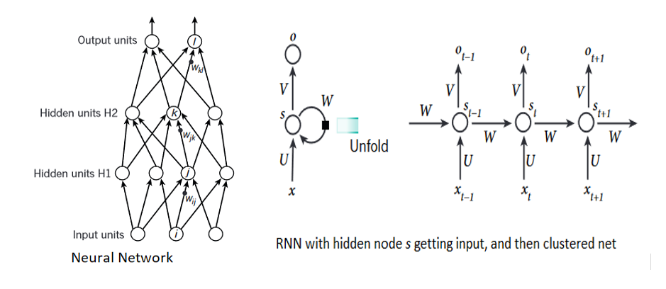
From the left side of image, we can understand that, both H1, and H2 hidden unit of neural network gets grouped together and hidden under node $s$ in RNN with value $s_{t}$ at time $t$ (LeCun, Bengio and Hinton, 2015). Also, we know that, each node in RNNs gets output from other neurons at the previous time step. It can be observed in the right side of the image that any output $o_{t+1}$ at any time step $t+1$ is influenced by all input values $x_{t}, x_{t+1}, \cdots x_{t-n}$ from previous time steps.
However, it is not enforced to follow the architecture on the right side, rigorously. RNNs architecture are can be of many types. Few are illustrated below in images:
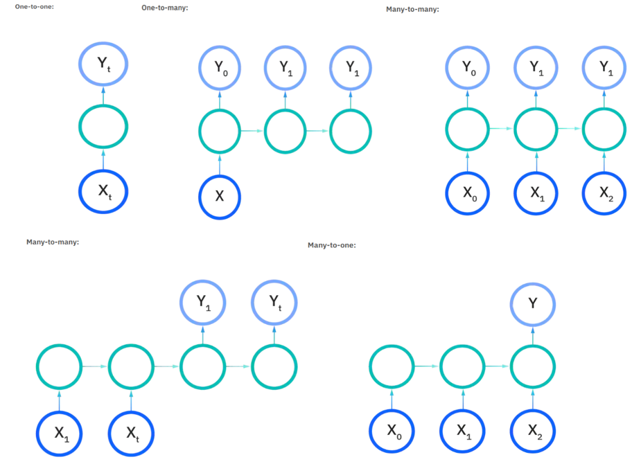
With these varied type of architecture RNNs get to learn long-term dependencies and becoming one of the efficient neural network and based on the problem at hand, one of RNNs architecture illustrated in images above can be used.
For instance, in the case of music-generation problem, one-to-many architecture could be used. On the other hand, in case of sentiment analysis, many-to-one RNN architecture would be suitable.
In general, RNNs architecture can be mathematical expressed as below:
\[X_{t} = W_{rec} σ (X_{t - 1}) + W_{In} \cdot u_{t} + b\]In the equation, $W_{rec}$ is recurrent weight, $\sigma$ is element-wise function, $W_{In}$ is input weight collected in $\theta$, $u_{t}$ is input, $b$ is bias, and $X_{t}$ is state at time $t$ (Pascanu, Mikolov, and Bengio, 2013).
Difficulty in Training RNNs
When Backpropagation Through Time (BPTT) was proposed, it was RNNs that got the best of it. However, while backpropagating through deep RNNs, exploding or vanishing gradients can hinder learning process as the same weight i.e., $W_{rec}$ is being shared by all the nodes in the architecture.
Let’s try to understand it well - In the above eq(1) of RNN architecture, we can understand that the cost function, $\displaystyle \epsilon = \sum_{1\le t \le T} ϵ X_{t}$ gets to measure the performance of some task, where $ϵ X_{t} = τ (x_{t})$ and therefore gradients for backpropagation can be expressed with:
\[\begin{equation} \large \frac{∂ \epsilon}{∂ \theta} =\sum_{1\le t\le T} \frac{∂ \epsilon_{t}}{∂ \theta} \end{equation}\] \[\begin{equation} \large \frac{∂ \epsilon_{t}}{∂ \theta}=\sum_{1\le k \le T}(\frac{∂ \epsilon_{t}}{∂ X_{t}}\cdot \frac{∂ X_{t}}{∂ X_{k}} \cdot \frac{\partial^+ X_{k}}{∂ \theta}) \end{equation}\] \[\begin{equation} \large \frac{\partial X_{t}}{\partial X_{k}} = \Pi_{t \ge i \gt k} \frac{\theta X_{i}}{\theta X_{i-1}} = \Pi_{t \ge i \gt k} \, W_{rec}^{T} \text{diag}(\sigma'(X_{i-1})) \end{equation}\]In eq(3) the gradient component $\displaystyle \frac{∂ \epsilon_{t}}{∂ \theta}$ is a sum of temporal contribution at given node. We can see that temporal contribution $\displaystyle \frac{∂ \epsilon_{t}}{∂ X_{t}} \cdot \frac{∂ X_{t}}{∂ X_{k}} \cdot \frac{\partial^{+} X_{k}}{∂ \theta}$ measures how $\theta$ at step $k$ affects the cost at step $t \lt k$. This gradient component $\displaystyle \frac{∂ \epsilon_{t}}{∂ \theta}$ transport the error in time from step $t$ back to step $k$. Next, we need to observe in the RHS of eq(4), here $W_{rec}^{T}$ is constant through all the time steps, and gets multplied with $diag$ that converts vector into diagonal matrix, and $\sigma’$ computing element-wise the derivative of $\sigma$.
Therefore,
If $W_{rec}$ is small, gradient starts to get smaller n smaller when pushed back into network, and neurons at earlier time steps fails to learn anything. This phenomenon is called Vanishing Gradient Problem
If $W_{rec}$ is large, backpropagating gradients start to grow exponentially. This is Exploding Gradient Problem.
Exploding gradient can be solved in two ways i.e., gradient scaling or gradient clipping.
In Gradient Scaling, we normalize/re-scale the error gradient vector norm if the vector norm crosses a certain threshold value, a value defined by us. On the other hand, in Gradient Clipping, if vector norm crosses the pre-defined threshold value, we force gradient values to a specific minimum or maximum value.
Vanishing gradient can be solved by slightly tweaked architecture of LSTM and GRU.
References
- Pascanu, R., Mikolov, T. and Bengio, Y., 2013, February. On the difficulty of training recurrent neural networks. In International conference on machine learning pp. 1310-1318.
- LeCun, Y., Bengio, Y. and Hinton, G., 2015. Deep learning. Nature, 521(7553), pp.436-444.