Activation Functions
In its simplest form, the neuron output of each layer is computed as: $a_{n+1} = w^T z_n + b_n$ where $w_n$ and $b_n$ are weight and bias parameters at layer $n$, respectively, and $z_n$ is neuron output of previous layer $n_1$ computed by a differentiable non-linear function $f(\cdot):z_n = f(a_n)$. This fixed non-linear function is known as activation function (Apicella et al., 2021).
Sigmoid, Hard-Sigmoid
The most common activation function is Sigmoid, also known as logistic. It is a bounded differentiable real-function defined as:
\[\text{Sigmoid} \quad or \quad σ = \frac{1}{1 + e^{-x}}\]Major problem with sigmoid is that, it binds all inputs between $0$ and $1$, where a large change of inputs leads to small change in output, resulting in smaller gradient values. When network is trained over many layers, these smaller gradient creates a vanishing gradient problem.
As a solution with Sigmoid, we have a Hard-Sigmoid which introduce linear behavior around $0$ to allow gradient flow easily. It can be defined as:
\[\text{Hard-Sigmoid}(x) = \begin{cases} 0, & \text{if $x \lt -2$} \\ \frac{1}{4}x + \frac{1}{2}, &\text{if -2 $\le$ x $\le$ 2} \\ 1, & \text{if x $\gt$ 2} \end{cases}\]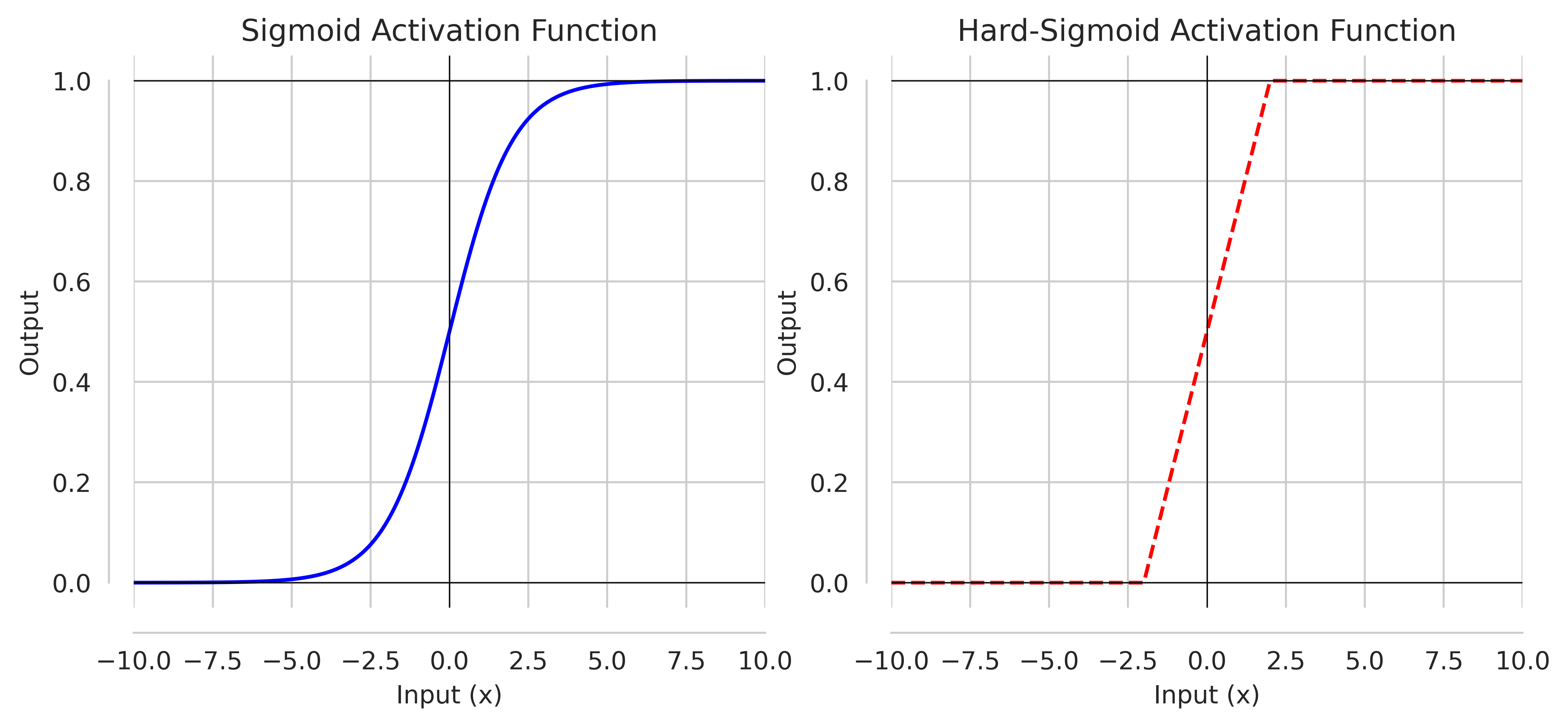
TanH, Hard-TanH
Hyperbolic Tangent (TanH) is similar to Sigmoid, continuous, bounded, differentiable and defined as:
\[\text{tanh} = \frac{e^{x} - e^{-x}}{e^{x} + e^{-x}}\]It has improved range of output i.e., between $-1$ to $1$. However, problem of large change of inputs leading to smaller change in output is not resolved, even with Hard-Tanh which can be expressed as:
\[\text{Hard-TanH}(x) = \begin{cases} -1, & \text{if $x \lt -1$} \\ x, &\text{if -1 $\le$ x $\le$ 1} \\ 1, & \text{if x $\gt$ 1} \end{cases}\]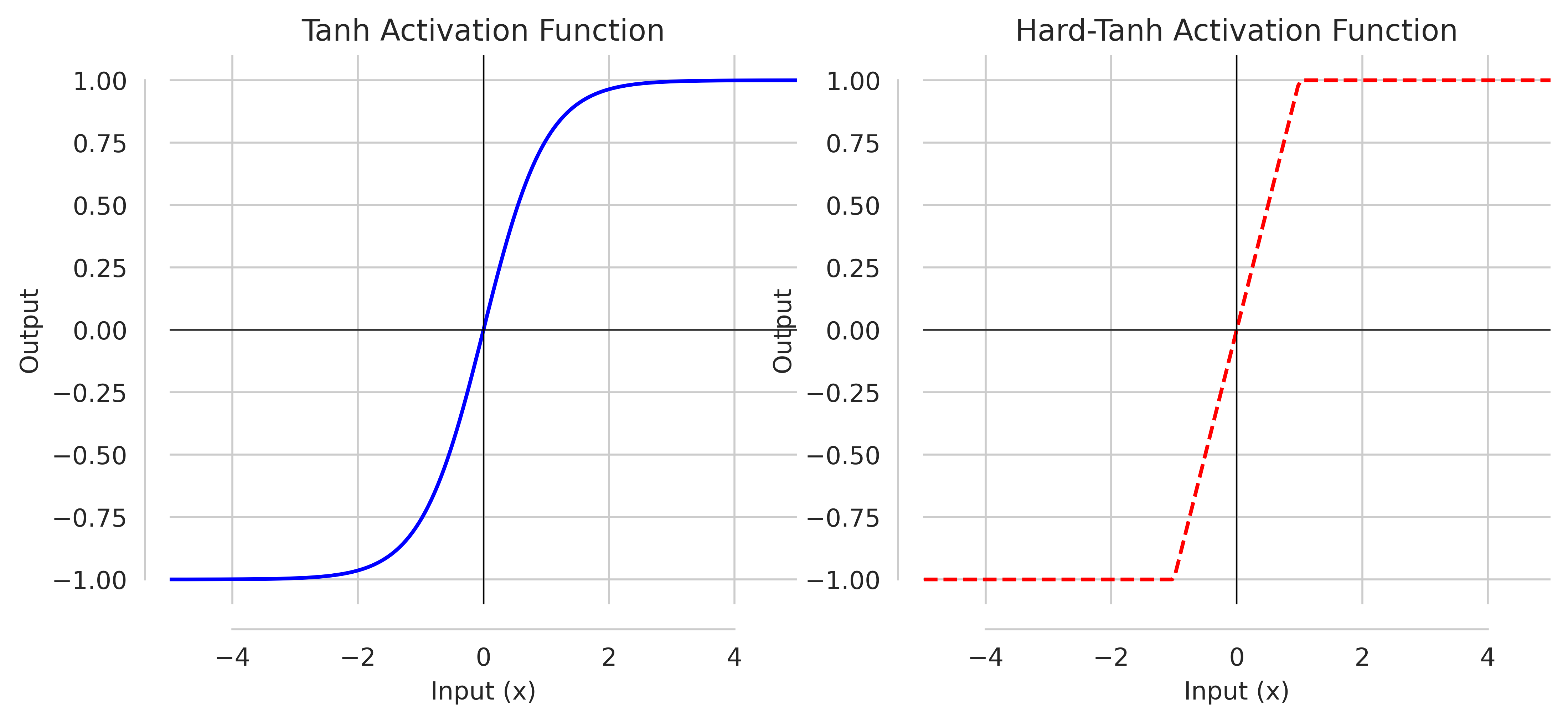
SoftSign
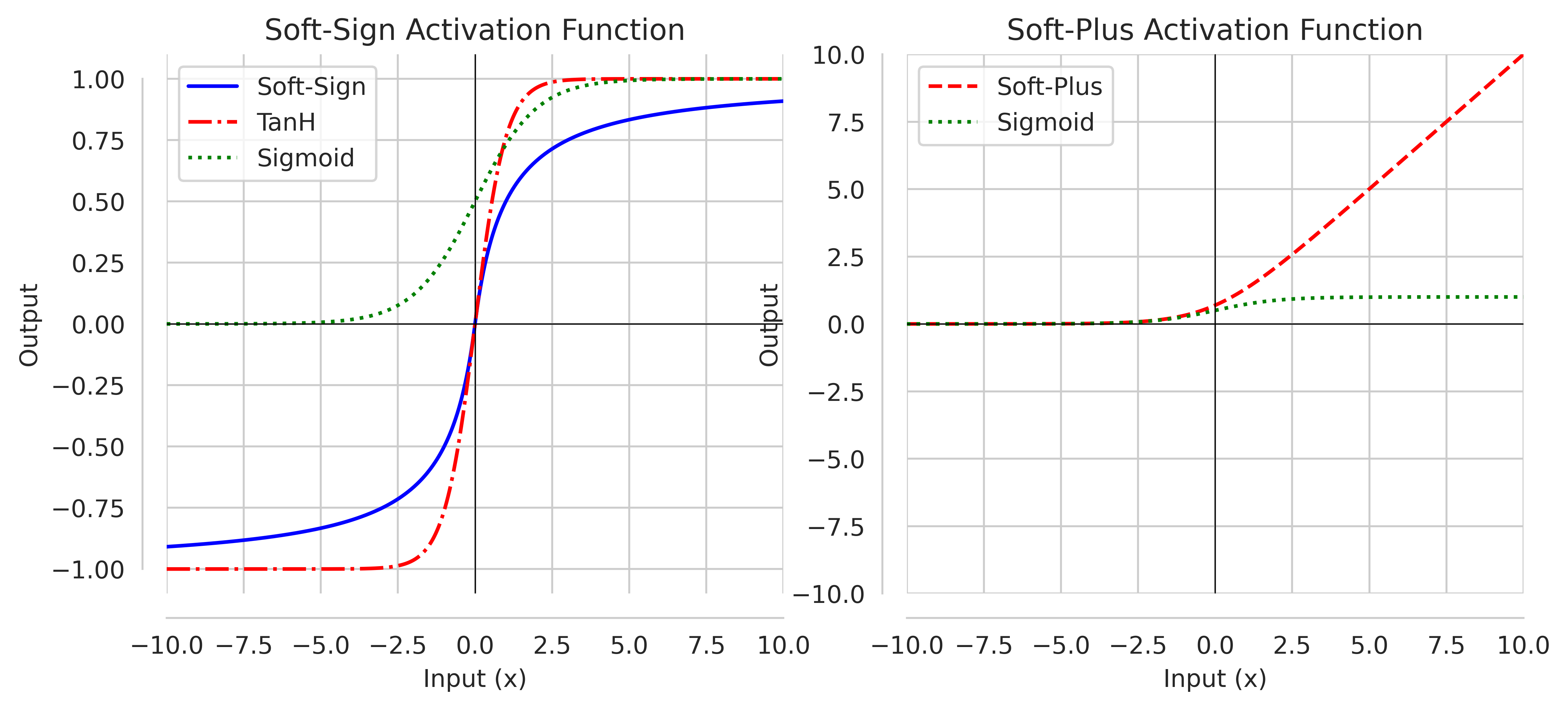
Softsign activation function is similar to Sigmoid (having “S”-shaped curve). It is also continuous, differentiable and can be defined as :
\[\text{SoftSign}(x) = \frac{x}{\lvert x \rvert + 1}\]If input is positive, SoftSign bind output between $0$ and $1$. However, it binds between $-1$ and $0$ for negative inputs.
Softplus
Another activation function similar to ReLU is softplus It is smooth approximation of ReLU function and defined as:
\[\text{softplus}(x) = \log(1 + \text{exp}(x))\]This was proposed to outperform ReLU, however results are more or less similar, with softplus being computationally costly.
ReLU
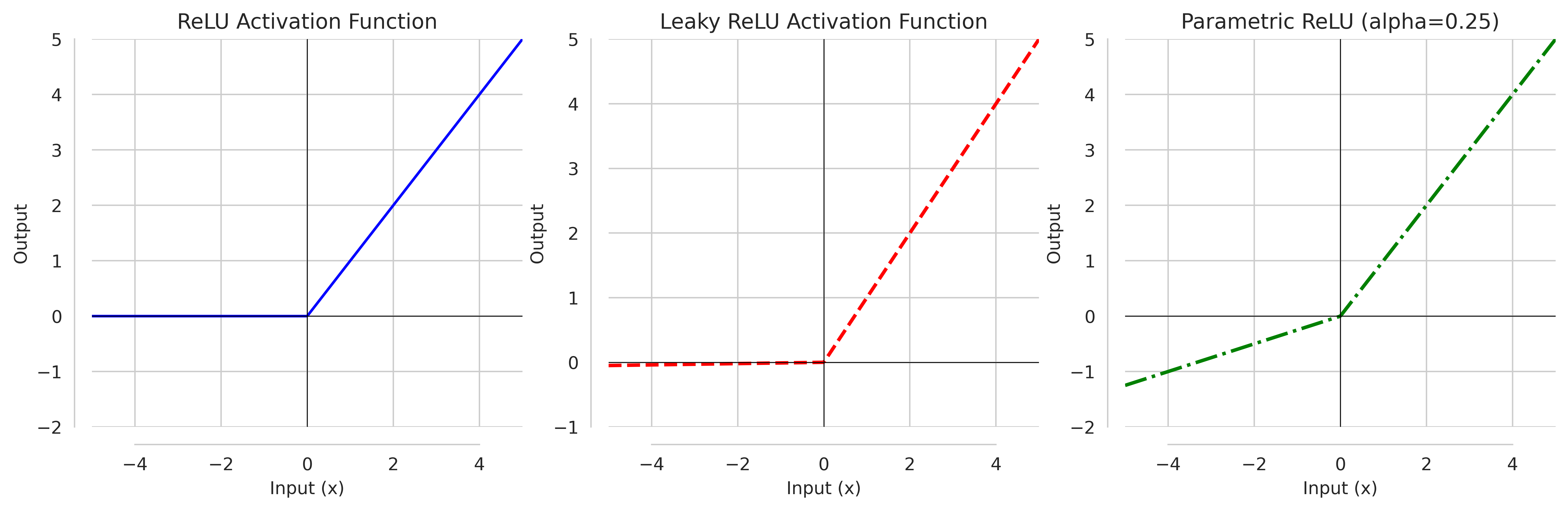
Rectified Linear Unit (ReLU) is continuous, non-bounded and unlike Sigmoid and Tanh, not-zero centered activation function that can be written as:
\[f(x) = \text{max}(0,x)\]It is not exponential, so computationally cheap, and alleviates the vanishing gradient problem for being not bounded in at least one direction. However, as negative inputs to ReLU evaluates to $0$, it start to create a problem to dead neuron
Leaky-ReLU, PReLU
Leaky-ReLU (LReLU)
It attempts to solve dead neuron issue with ReLU by allowing small gradient to flow when inputs are non-positive. It can defined as:
\[\text{LReLU}(x) = \begin{cases} x, & \text{if $x \ge 0$} \\ 0.01 ⋅ x, & \text{otherwise} \end{cases}\]However, it does not bring significant improvement, rather possibility of vanishing gradient problem coming back.
Parametric ReLU (PReLU):
PReLU attempts to resolve Leaky-ReLU problem by taking additional parameter $\alpha$. This additional parameter is learnt jointly with whole model using gradient method without weight decay(to not push $\alpha$ to zero). It can be defined as:
\[\text{PReLU}(x) = \begin{cases} x, & \text{if $x \ge 0$} \\ \alpha ⋅ x, & \text{otherwise} \end{cases}\]It is not computationally expensive to ReLU or Leaky-ReLU and slightly improves on vanishing gradient. With, PyTorch default of alpha = 0.25 for $\text{PReLU}$, we have below given illustration.
Exponential Linear Units (ELU), PELU, SELU
It is another method similar to ReLU (or parametric ReLU). It can be defined as:
\[\text{ELU}(x) = \begin{cases} x, & \text{if $x \ge 0$} \\ \alpha ⋅ (\text{exp}(x) -1), & \text{otherwise} \end{cases}\]With the additional parameter $\alpha$ controlling the values for negative inputs, ELU allows faster learning as values given by ELU units push the mean of activation closer to $0$.
Parametric Exponential Linear Units (PELU)
PELU takes two trainable parameter, that do not need to be manually set, learned with other network parameters using gradient method. It can be defined as :
\[\text{PELU}(x) = \begin{cases} \frac{\beta}{\gamma}x, & \text{if $x \ge 0$} \\ \beta ⋅ (\text{exp}(\frac{x}{\gamma}) -1), & \text{otherwise} \end{cases}\]Scaled Exponential Linear Units (SELU)
SELU has additional scaling hyper-parameter $\lambda$. It can be defined as:
\[\text{SELU}(x) = λ \begin{cases} x, & \text{if $x \ge 0$} \\ \alpha ⋅ (\text{exp}^x -1), & \text{otherwise} \end{cases}\]Here, $λ ≈ 1.05070098$, and $α ≈ 1.67326324$. SELU is effective when it comes to covariate shift, and vanishing / exploding gradient problem for having self-normalizing property. By self-normalizing, we mean if the SELU inputs follows a Gaussian distribution with mean and variance around $0$ and $1$, respectively, the mean and variance of SELU are also around $0$ and $1$.
SiLU
Sigmoid-weighted Linear Units (SiLU)
SiLU is sigmoid function weighted by its inputs, so can be expressed as:
\[\text{SiLU}(x) = x ⋅ \text{sigmoid}(x)\]Swish Activation, E-Swish
Swish is another function based on Sigmoid, but similar to ReLU for being unbounded above and bounded below. However, unlike ReLU, Swish is non-monotonic, and smooth. It can be defined as:
\[\text{Swish}(x) = x ⋅ \text{Sigmoid}{β ⋅ x}\]They key thing with Swish is when trainable parameter $\beta$ approaches $\infty$, it behaves like ReLU, and when $β = 1$, it is similar to SiLU. (Ramchandran, Zoph & Le, 2017)
E-Swish
E-Swish is similar to SiLU, but with additional parameter that needs to be tuned by user. It can be written as:
\[\text{E-Swish}_{\gamma}(x) = γ x ⋅ \text{sigmoid}(x)\]Mish Activation
Mish is similar to Swish, smooth, continuous, non-monotonic, unbounded above and bounded below. It can be defined as:
\[\text{Mish}(x) = x \text{tanh}(\text{softplus}(x))\]It is effectively solving dead neuron and vanishing gadient problem, and usually outperform Swish, and ReLU.
Gaussian Error Linear Units (GELU)
GELU is one of the most promising activation function. It is widely used in BERT, GPT-3 and other transformers. GELU weight inputs by their values, rather than gated sign as in ReLU. GELU scales input $x$ by how much greater it is than other inputs. It can be expressed as:
\[\text{GELU}(x) = x ⋅ Φ (x) \notag\]Where, $\Phi(x)$ is cumulative distribution function of standard Gaussian distribution. Thus, GELU can be defined as:
\[\text{GELU}(x) = x ⋅ \frac{1}{2}\left[1 + \text{erf}(x / \sqrt{2}) \right]\]GELU can be approximated with $0.5\,x(1 + \text{tanh}[\sqrt{\frac{2}{\pi}}(x + 0.044715x^3)])$ (Hendrycks & Gimpel, 2016)
Optimization Methods
Gradient Descent
Gradient Descent or Batch Gradient Descent is a way to minimize the objective (cost) function \(J(\theta)\) parameterized by model’s parameters \(θ ∈ \mathbb{R}^d\) by updating the parameters in the opposite direction of the gradient of the objective function \(\Delta_{\theta}J(\theta)\) w.r.t to the parameters for the entire dataset.
Parameter update rule can be written as:
\[θ = θ - η ⋅ \Delta_{\theta} J(\theta)\]Where $\eta$ is the learning rate determining the size of the step we take to reach a (local) minimum. Gradient Descent method is slow and intractable for calculating all the gradients of training examples before making one update.
Stochastic Gradient Descent
Stochastic Gradient Descent (SGD) resolves it by performing a parameter update for each training example \((x^{(i)},y^{(i)})\)
\[θ = θ - η ⋅ \Delta_{\theta} J(\theta, x^{(i)}, y^{(i)})\]Updating parameters for each training examples makes it faster, but with higher variance, therefore SGD can overshoot the exact covergence to the global minimum.
Mini-Batch Gradient Descent
Mini-Batch resolves the high variance problem with SGD by performing update on parameters on every mini-batch of $n$ training examples.
\[θ = θ - η ⋅ \Delta_{\theta} J(\theta, x^{(i:i+n)}, y^{(i:i+n)})\]Mini-batch can be of range 50-256.
Momentum
Momentum resolves the slow convergence to global minimum problem with SGD by adding a fraction $\gamma$ of the previous update vector to the current one. The momentum term $γ$ is set to 0.9 or similar value.
The equation used to update parameter with Momentum method is as follows:
\[v_t = γ v_{t-1} + η ⋅ \Delta_{\theta} J(\theta)\] \[θ = θ - v_t\]Here, $v_t$ is current update vector, $v_{t-1}$ is the previous vector, $\theta$ is the parameters we are optimizing for, $\eta$ is the learning rate, $\Delta_{\theta}J(\theta)$ is gradient of objective function $J(\theta)$ w.r.t. $\theta$
Momentum, thus, helps to increase the step size in dimensions where the gradient is consistently pointing in the same direction (accelerating towards convergence), and reduces the step size in dimensions where the gradient frequently changes directions.
Nesterov Accelerated Gradient
Nesterov Accelerated Gradient (NAG) is further improvement on Momentum method. It gives an approximation of the next position of parameters by computing $θ - γ v_{t-1}$. We can then calculate the gradient not w.r.t to our current parameters, but w.r.t to the approximate future position of our parameters as follows:
\[v_t = γ v_{t-1} + η \Delta_{\theta} ⋅ J(θ - γ v_{t-1})\] \[θ = θ - v_t\]The momentum term $\gamma$ again can be set to 0.9 or similar value.
AdaGrad
In AdaGrad method, we adapt the learning rate to the parameters, performing larger updates from infrequent parameters, and smaller updates for frequent ones. This is achieved by introducing per-parameter learning rate for each time step. The update rule is as follows:
\[\theta_{(t+1),i} = \theta_{t,i} - \frac{\eta}{\sqrt{G_{t,ii} + \epsilon}} ⋅ g_{t,i}\]where,
$g_{t,i}$ is the gradient of the objective function w.r.t. the parameters $\theta_{i}$ at time step $t$ i.e, $g_{t,i} = \Delta_{\theta_{t}} J(\theta_{t,i})$.
$\eta$ is the initial learning rate,
$\epsilon$ is the smooting term to avoid division by zero (usually on the order of 1e-8)
$G_t ∈ \mathbb{R}^{d× d}$ is the diagonal matrix each diagonal element $i,i$ is the sum of squares of gradients w.r.t $\theta_{i}$ across all previous time step.
If $G_{t,ii}$ is smaller, parameters had not had many updates, and learning rate can stay relatively larger, but when $G_{t,ii}$ gets large, learning rate becomes smaller - slowing down updates on that parameters.
We can further vectorise AdaGrad as following, instead of treating for each parameter.
\[\theta_{t+1} = \theta_{t} - \frac{\eta}{\sqrt{G_{t} +\epsilon}} ⊙ g_{t}\]AdaGrad is highly suitable for modelling with sparse data, and learning rate tuning is not necessary, and negative aspect of AdaGrad is that it can shrink learning rate over time, for accumulating positive terms in the denominator of eq(25) and eq(26).
Adadelta
AdaDelta removes drawbacks in AdaGrad i.e, (1) need to select global learning rate at the beginning, and (2) its continual decay over time.
It can be achieved by restricting the window of past squared gradients at some $w$, however to make it more efficient, the sum of gradients is recursively defined as a decaying average of all past squared gradients. If at any given time $t$, this running average is $\mathbb{E}[g^2]_t$, then we can calculate it as:
\[\mathbb{E}[g^2]_t = ρ \mathbb{E}[g^2]_{t-1} + (1-\rho)g^2_t\]here, $\rho$ is a decay constant similar to momentum $\gamma$ and can be set to 0.9 or similar value.
The parameter update vector of Adadelta now will take the same form of Adagrad in eq$(26)$ in which we will replace diagonal matrix $G_t$ with the decaying average of past squared gradients $\mathbb{E}[g^2]_t$. It is expressed as:
\[Δ \theta_{t} = -\frac{\eta}{\sqrt{\mathbb{E}[g^2]_t + \epsilon}}⋅ g_t\]As the denominator is just the root mean squared (RMS) error criterion of the gradient, we can further improve last eq$(28)$ as:
\[Δ \theta_{t} = -\frac{\eta}{\text{RMS}[g]_t}⋅ g_t\]Another key thing - as units in the above update do not match, Adadelta defines another decaying average of squared parameters, instead of squared gradients, as:
\[\mathbb{E}[Δ \theta^2]_t = ρ \mathbb{E}[Δ \theta^2]_{t-1} + (1 - \rho)Δ \theta^2_t\]Therefore, Root Mean Square of parameter is following:
\[\text{RMS}[Δ \theta]_t = \sqrt{\mathbb{E}[Δ \theta^2]_t + \epsilon}\]However, \(\text{RMS}[Δ θ]_t\) is unknown, so we approximate it with the RMS value up to the previous time step \(t-1\), denoted as \(\text{RMS}[Δ θ]_{t-1}\). We can replace the learning rate \(\eta\) with this approximation, making the Adadelta update rule as follows:
\[Δ θ_{t} = - \frac{\text{RMS}[Δ \theta]_{t-1}}{\text{RMS}[g]_t} ⋅ g_{t}\] \[\theta_{t+1} = \theta_{t} + Δ \theta_{t}\]Adadelta do not need learning rate to be specified, as evident in the update rule.
RMSProp
Root Mean Square Propagation (RMSProp) is to resolve the issues with AdaGrad. Adadelta and RMSProp are both similar method solving similar problem.
RMSprop, however, stops at eq (28) where we replace the diagonal matrix $G_t$ in the update rule with decaying average of past squared gradients as:
\[Δ \theta_{t} = -\frac{\eta}{\sqrt{\mathbb{E}[g^2]_t + \epsilon}}⋅ g_t\]RMSProp, afterwards, does not track the running average of squared parameters updates to tackle mis-match in unit-consistency. RMSProp, on the other hand, requires learning rate to be provided to its update rule. Default learning rate can be used as 0.001
ADAM
Adaptive Moment Estimation (ADAM) estimates the first moment (mean) of the past gradient similar to Momentum, and second moment (uncentered variance) of the past squared gradients similar to Adadelta/RMSProp.
First moment is represented by $m_t$ and second by $v_t$ where the hyper-parameters \(\beta_1, \beta_2 ∈ [0,1)\) control the exponential decay rates of these moving averages.
\[m_t = β_1 m_{t-1} + (1 - β_1)⋅ g_t\] \[v_t = β_2 m_{t-1} + (1 - β_2)⋅ g^2_t\]However, both $m_t$ and $v_t$ are biased towards zero for being initialised as 0. So, we counter it by bias-correct measure as mentioned below:
\[\hat{m_t} = \frac{m_t}{1 - \beta^t_1}\] \[\hat{v_t} = \frac{v_t}{1 -\beta^t_2}\]Then, we can write final update for the ADAM method as following:
\[\theta_t = \theta_{t-1} - α ⋅ \frac{\hat{m_t}}{\sqrt{\hat{v_t} + \epsilon}}\]Here, α is the stepsize, can be used at 0.001, $\epsilon$ is correction term with value \(\text{1e-8}\), $\beta_1 = 0.9$ and $\beta_2 = 0.999$
Adamax
Adamax is further improvement on ADAM as the $v_t$ factor in the update rule scales the gradient inversely proportional to the $L^2$ norm of the past gradient at $v_{t-1}$ and current gradient at $v_t$.
We can, however generalize the $L^2$ norm based update rule to a $L^P$ norm based update rule, and as $L → ∞$ algorithm stabilies, so we can improve on ADAM as below:
\[v_t = \beta^p_2 v_{t-1} + (1 - \beta^p_2)\lvert g_t \rvert^p\] \[\qquad = (1 - \beta^p_2) \sum_{i=1}^t \beta^{p(t-i)}_2 ⋅ \lvert g_i \rvert^p\]For distinction, we use, $u_t$ for the second moment in Adamax, and ensure update reflect largest of past accumulated gradient or current gradient by taking maximum value of them as follows:
\[u_t = \text{max}(\beta_2 ⋅ u_{t-1}, \lvert g_t \rvert)\]Thus, we can write the update rule for Adamax as given below:
\[θ_t = θ_{t-1} - \left(\frac{\alpha}{1 - \beta^t_1}\right) ⋅ \frac{m_t}{u_t}\]Here, $\left(\frac{\alpha}{1 - \beta^t_1}\right)$ is the learning rate with the bias-corrected term for the first moment. Good values for $α$ is 0.002, $\beta_1 = 0.9$ and $β_2 = 0.999$
Adafactor
Adafactor further improving on ADAM, reducing computation cost by tracking moving averages of rows and column sum of squared gradients for matrix-valued variables, instead of maintaining $V ∈ \mathbb{R}^{n× m}$ of squared gradients. This reduces memory cost to $n + m$ instead of $n × m$.
We split second-moment into row-wise and column-wise components as:
\[R_t = \hat{\beta}_{2t}R_{t-1} + (1 - \hat{\beta}_{2t})(G^2_t + \epsilon_1 1_n 1^T_m)\] \[C_t = \hat{\beta}_{2t}C_{t-1} + (1 - \hat{\beta}_{2t})1^T_n(G^2_t + \epsilon_1 1_n 1^T_m)\]Here, $R_t$ is a vector of size $n$ for row-wise second moment $C_t$ is a vector of size $m$ for column-wise second moment. \(G^2_t\) is squared gradient i.e, \(G^2_t = (Δ f_t (X_{t-1}))^2\). $\epsilon_1$ is regularizing constant to avoid 0, and suggested $\epsilon_1 = 10^{-30}$ and $\hat{\beta}_{2t} = 1 - t^{-0.8}$
Next, we deduce low-ranking approximation for second moment as:
\[\hat{V}_t = \frac{R_t C_t}{1^T_n R_n}\]Adafactor also proposed Gradient Clipping
One problem with ADAM optimizer is that it fails to convergence in fast-decay of squared gradients, and becomes unstable with slow decay. We measure this by calculating root mean square (RMS) over all parameters $x$ in weight matrix / vector for a given time-step $t$ of unscaled parameter update i.e.,
\[U_{t} = -\frac{G_{t}}{\sqrt{\hat{V}_{t}}}\]For clarity, it is called RMS and can also be expressed as:
\[\text{RMS}(U_t) = \text{RMS}_{x∈X} (u_{xt}) = \sqrt{\text{Mean}_{x∈X}\left(\frac{(G_t)^2}{\hat{V}_{t}}\right)}\]- If $\text{RMS}(U_t) \gt 1$. The updates are too large, and can lead to instability
- If $\text{RMS}(U_t) \lt 1$. The updates are too small, and can lead to non-convergence
Gradient Clipping with threshold $d$ is introduced to resolve this problem scaling down on update of weight vector/matrix. Hence, we can write clipped unscaled update $\hat{U}_t$ as :
\[\hat{U}_t = \frac{U_t}{\text{max}(1, RMS(U_t)/d)}\]Adafactor uses relative step size over absolute step size. We get it by multiplying with the scale of parameters i.e, RMS of its component from previous time step. It is also lower-bounded by small $\epsilon_2$ to escape 0. We can express this as:
\[\alpha_t = \text{max}(\epsilon_2, \text{RMS}(X_{t-1}))⋅ \rho_t\]Here, proposed hyper-parameter for $d = 1$ in eq(49) and for eq(50)$\rho_t = \text{min}\left(10^{-2},\frac{1}{\sqrt{t}}\right)$, $\epsilon_2 = 10^{-3}$. With all the values obtained above, we can finally express our update rule for AdaFactor as:
\[X_t = X_{t-1} - \alpha_t \hat{U}_t\]AMSGrad
Nadam
LION
Loss Functions
References
- Apicella, A., Donnarumma, F., Isgrò, F. and Prevete, R., 2021. A survey on modern trainable activation functions. Neural Networks, 138, pp.14-32.
- Hendrycks, D. and Gimpel, K., 2016. Gaussian error linear units (gelus). arXiv preprint arXiv:1606.08415.
- Hinton, G., Srivastava, N. and Swersky, K., 2012. Neural networks for machine learning lecture 6a overview of mini-batch gradient descent. Cited on, 14(8), p.2.
- Kingma, D.P., 2014. Adam: A method for stochastic optimization. arXiv preprint arXiv:1412.6980.
- Ramachandran, P., Zoph, B. and Le, Q.V., 2017. Searching for activation functions. arXiv preprint arXiv:1710.05941.
- Reddi, S.J., Kale, S. and Kumar, S., 2019. On the convergence of adam and beyond. arXiv preprint arXiv:1904.09237.
- Ruder, S., 2016. An overview of gradient descent optimization algorithms. arXiv preprint arXiv:1609.04747.
- Shazeer, N. and Stern, M., 2018, July. Adafactor: Adaptive learning rates with sublinear memory cost. In International Conference on Machine Learning (pp. 4596-4604). PMLR.
- Wang, Q., Ma, Y., Zhao, K. and Tian, Y., 2020. A comprehensive survey of loss functions in machine learning. Annals of Data Science, pp.1-26.
- Zeiler, M.D., 2012. ADADELTA: an adaptive learning rate method. arXiv preprint arXiv:1212.5701.