Self-supervised learning is a deep learning method in which a model learns representation form unlabeled data. It leverages data’s inherent co-occurence relationship or lack thereof as self-supervision for labels (Liu et al., 2021). Yann LeCun put it as, “the machine predicts any parts of its input for any observed part”
Self supervised learning can be summarized as:
- Obtain “labels” from data itself by using internal structure
- Predict part of the data from the other parts, where other parts could be incomplete, transformed, distorted or corrupted (Liu et al., 2021)
For ease of purposes, we can separate self-supervised learning into three categories:
- Generative : In this, we have an encoder and a decoder. We encode an input \(x\) into an explicit vector \(z\) and using reconstruction loss, decoder afterwrads tries to reconstruct \(x\) from \(z\). Generative methods are AutoEncoder and its variants
- Contrastive : In contrastive learning, we have an encoder, and a discriminator. Here, we encode an input $x$ into an explicit vector \(z\).Discriminator then uses similarity metrics such as InfoNCE to maximize the similarity between positive samples, and minimize the similarity between negative samples.
- Generative - Constrastive : Here, we have an encoder-decoder where $z$ implicitly modelled to generate fake samples, and then a discriminator using distribution divergence loss such JS-Divergence, Wasserstein Distance tries to distinguish fake samples from the real ones. GAN and its variants fall into this category.
Contrastive Learning
There are many ways to approach contrastive learning problem. One of them is Mutual Information.
Mutual Information (MI) measures the degree of dependence or correlation between the input data and the learned representation. The goal is to maximize the MI between input data and learned representation where positive pairs share more MI than negative pairs.
If \(p(x)\) is the data distribution
\(p(x, c)\) is the joint distribution for data and representation
\(p(c)\) is the marginal distribution of the representations
and \(X\) and \(C\) are the random variables associated with data and representations, respectively.
Then Mutual Information (MI) (Song and Ermon, 2020) can be given as:
\[I(X, C) ≔ \mathbb{E}_{(x, y) ∼ p(x,y)} \left[\log \frac{p(x,c)}{p(x)p(c)}\right]\]Contrastive Predictive Coding
One of the approach that uses MI is Contrastive Predictive Coding (CPC).
In CPC, a non-linear encoder \(g_{\text{enc}}\) maps the input data sequences $x_t$ to latent representations \(z_t = g_{\text{enc}}(x_t)\). Then, an autoregressive model \(g_{\text{ar}}\) summarizes all \(z_{\le t}\) and produces a latent representation \(y_t = g_{\text{ar}}(z \le t)\) (Oord et al., 2019) as shown in the image below:
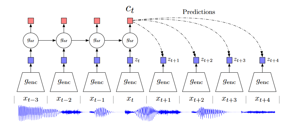
Then, if that CPC is an $m$-class classification problem, wher the goal is to distinguish a positive pair \((x, c) ∼ p(x, c)\) from \((m -1)\) negative pair \((x, c̄ ) ∼ p(x)p(c)\).
We optimize the loss for a batch of \(n\) positive pairs \({(x_{i}, c_{i})}_{i=1}^{n}\) as:
\[L(g) ≔ \mathbb{E} \left[\frac{1}{n} \sum\limits_{i=1}^{n} \log \frac{m ⋅ g(x_{i},c_{i})}{g(x_{i}, c_{i}) + \sum\limits_{j=1}^{m-1} g(x_{i}, c_{i,j})}\right]\]This loss function is called Information Noise Contrastive Estimation or InfoNCE and used in many further proposed methods in Contrastive Learning.
Both encoder and autoregressive model jointly optimize the loss using InfoNCE, and CPC afterwards models a density ratio which preserves the Mutual Information between \(x_{t+k}\) and \(c_t\) (Oord et al., 2019) as follows :
\[f_{k}(x_{t+k},c_{t}) ∝ \frac{p(x_{t+k} ∣ c_{t})}{p(x_{t+k})}\]In CPC, both \(z_t\) and \(c_t\) can be used as representation for downstream task, when more information from past is necessary \(c_t\) is suitable.
Contrastive Multiview Coding
(Tian et al., 2020)
SimCLR
SimCLR is one of the simplest yet effective method proposed for contrastive learning of visual representations. Key features of simCLR framework are :
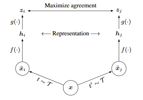
- Data Augmentation: Using stochastic data augmentation, first two correlated data samples are generated from one, as \(\widetilde{x_{i}}\) and \(\widetilde{x_{j}}\).
-
Encoder: A neural network base encoder \(f(⋅)\) is used to map augmented data samples to a lower-dimensional representation. SimCLR used ResNet (Chen et al., 2020) to obtain \(h_{i} = f(\widetilde{x_{i}}) = \text{ResNet} (\widetilde{x_{i}})\) where \(h_{i} ∈ \mathbb{R}^{d}\) is the ouput after the average pooling layer.
-
Projection Head: Afterwards, a small neural network projection head \(g(\cdot)\) is used with one hidden layer to obtain latent space \(z_{i}\) where, \(z_{i} = g(h_{i}) = W^{2}σ (W^{1}h_{i})\) where \(σ\) is a ReLU function. It is beneficial to maximize agreement using contrastive loss on \(z_{i}\) than \(h_{i}\).
- Contrastive Loss Function : Given a set of \(\left\{\widetilde{x_{k}}\right\}\) including positive pair of \(\widetilde{x_{i}}\) and \(\widetilde{x_{j}}\), it aims to identify \(\widetilde{x_{j}}\) in \(\left\{\widetilde{x_{k}}\right\}_k ≠ i\). SimCLR framework is illustrated in the image below :
SimCLR Optimization Process
For the optimization in SimCLR, we have a minibatch of $N$ data samples which gets augmented into \(2N\) samples. Negative data example are not explicitly sampled, but given a positive pair, remaining \(2(N-1)\) are treated as negative ones.
The loss function of positive pair of examples \((i,j)\) is defined as:
\[l_{(i,j)} = -\log \frac{\text{exp}(\text{sim}(z_{i},z_{j})/ τ)}{\sum\limits_{k=1}^{2N} 1_{k ≠ i} \text{exp}((z_{i}, z_{k}) / τ)}\]where,
\(\text{sim}(⋅, ⋅)\) is cosine similarity function i.e, \(\text{sim}(u, v) = \frac{u^{T} v} {\lVert u \rVert \, \lVert v \rVert}\) to normalize the representation. \(\tau\) is a temperature parameter. \(1_{k ≠ i} ∈ \left\{0, 1\right\}\) is an indicator function if and only if \(k ≠ i\)
The final loss is computed as :
\[\mathfrak{L} = \frac{1}{2N} \sum\limits_{k=1}^{N} \left[l(2k-1, 2k) +l(2k, 2k-1)\right]\]and is called NT-Xent (Normalized Temperature Scaled Cross Entropy Loss)
References
-
Liu, X., Zhang, F., Hou, Z., Mian, L., Wang, Z., Zhang, J. and Tang, J., 2021. Self-supervised learning: Generative or contrastive.IEEE transactions on knowledge and data engineering, 35(1), pp.857-876.
- Oord, A.V.D., Li, Y. and Vinyals, O., 2018. Representation learning with contrastive predictive coding. arXiv preprint arXiv:1807.03748.
- Song, J. and Ermon, S., 2020. Multi-label contrastive predictive coding. Advances in Neural Information Processing Systems, 33, pp.8161-8173.
- Chen, T., Kornblith, S., Norouzi, M. and Hinton, G., 2020, November. A simple framework for contrastive learning of visual representations. In International conference on machine learning (pp. 1597-1607). PMLR.