Deep Q-Learning
In \(Q-\)Learning, representing the \(Q-\)function as a table for all state-action pairs can be impractical. Deep Q-Learning solves this by training a neural network with parameters \(θ\) to approximate \(Q-\)values i.e., \(Q(s,a; θ) ≈ Q^{\ast}(s,a)\).
This is achieved by minimizing loss at each time step \(t\), enabling efficient estimation of \(Q-\)values without an exhaustive table representation.
In addition, Deep Q-Learning uses a technique called Experience Replay during network updates. In this technique, at each time step \(t\), the transitions are added to a circular buffer called replay buffer. During training, instead of using only the most recent action, a mini-batch of transitions sampled from the replay buffer is employed to compute the loss and its gradient, improving learning efficiency and stability.
Deep Q-Learning Steps
Initializtion:
- Experience replay is initialized to an empty list of size \(M\).
2.We choose a maximum size of the memory.
At each time step \(t\), we repeat then following processes until the end of the epoch.
-
We predict the \(Q-\)values of the current state \(s_{t}\).
-
We play the action that has the highest \(Q-\)value: \(a_{t} = \text{arg} \text{max}_{a}{Q(s_{t},a)}\).
-
We get the reward \(R(s_{t},a_{t})\).
-
We reach the next state \(s_{t+1}\).
-
We append the transition \((s_{t},a_{t},r_{t},s_{t+1})\) in the memory \(M\).
-
We take a random mini-batch \(B \subset M\) of replay buffer. For all the transitions \((s_{t_{B}},a_{t_{B}},r_{t_{B}},s_{t_{B+1}})\) of the random mini-batch \(B\).
We get the predictions, \(Q(s_{t_{B}},a_{t_{B}})\).
We get the target \(R(s_{t_{B}},a_{t_{B}}) + \gamma \text{max}_{a} (Q(s_{t_{B+1}},a))\).
Now, we compute the desired loss between the predictions and target over the whole mini-batch \(B\).
\[\begin{align} \text{Loss} &= \frac{1}{2} \sum\limits_{B} (R(s_{t_{B}},a_{t_{B}}) + \gamma max_{a} (Q(s_{t_{B+1}},a)) - Q(s_{t_{B}},a_{t_{B}}))^{2}\notag\\ &= \frac{1}{2}\sum\limits_{B} TD_{t_{B}}(s_{t_{B}},a_{t_{B}})^{2}\notag\\ \end{align}\]Afterwards, we backprop the loss error back into network, and through stochastic gradient descent, we update the weights on network.
Double Q-Learning
In Q-Learning, update can be written as:
\[Q_{t+1}(s_{t},a_{t}) = Q_{t}(s_{t},a_{t}) + \alpha_{t}(s_{t},a_{t})(R_{t} + \gamma max_{a} Q_{t}(s_{t+1},a) - Q_{t}(S_{t},a_{t}))\]The use of max operator in the above eq of Q-Learning, can cause large over-estimation of the action values. This leads to large performance penalty that slows the learning process too.
Therefore, Double Q-Learning proposes the double estimator method. Here, two sets of estimators: \(μ^{A} = {\mu_{1}^{A},\cdots, \mu_{M}^{A}}\) and \(\mu^{B} = {\mu_{1}^{B},\cdots, \mu_{M}^{B}}\) is used to approximate \(max_{i}E\left\{X_{i}\right\}\). The approximation can be written as :
\[max_{i}E\left\{X_{i}\right\} = max_{i}E\left\{\mu_{i}^{B}\right\} ≈ \mu_{a\ast}^{B}\]Double Q-Learning Method
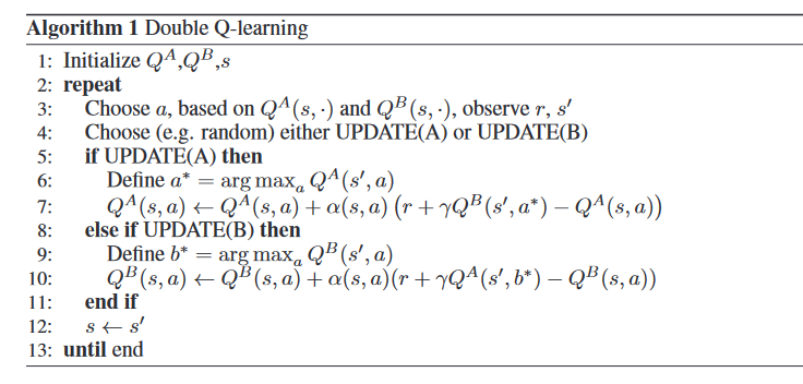
It stores two \(Q\) functions: \(Q^{A}\) and \(Q^{B}\). Each \(Q\) function is updated with a value from the other \(Q\) function for the next state. This way it can be considered an unbiased estimate for the value of this action.
For instance, the action \(a^{\ast}\) in eq(3) is the maximum value action in state \(s^{'}\), according to the value function \(Q^{A}\). i.e, \(Q^{A}(s^{'},a^{\ast}) = max_{a}Q^{A}(s^{'},a)\). However, we still use \(Q^{B}(s^{'},a^{\ast})\) to update \(Q^{A}\).
Double Q-Learning converges to the optimal policy in the limit, and faster than Q-Learning, its algorithm is given below :