U-Net
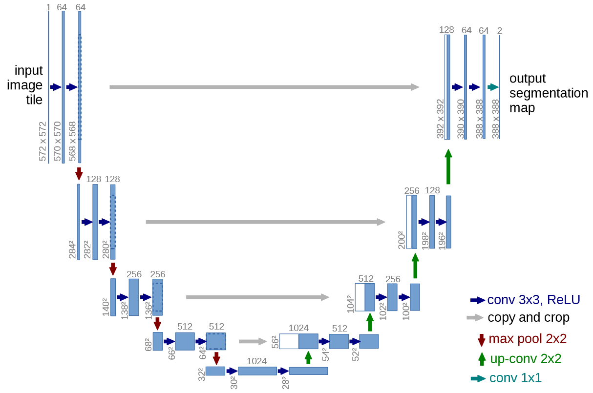
U-Net architecture consists of a contracting path that downsamples the input image through a series of convolutional layers, increasing number of channel and extracting feature maps at different scales, and an expansive path that upsamples these feature representations from the bottleneck layer decreasing number of channels, and increasing scale. The upsampling layers also concatenate its corresponding features from the contracting path, in order to retain spatial information (Ronneberger et al. 2015). Architecture of U-Net is attached below:

U-net architecture (example for 32x32 pixels in the lowest resolution). Each blue box corresponds to a multi-channel feature map. The number of channels is denoted on top of the box. The x-y-size is provided at the lower left edge of the box. White boxes represent copied feature maps. The arrows denote the different operations.
- Contracting path consists of many layers of repeated sequences of $3 × 3$ unpadded convolutional layers, followed by a ReLU unit and a $2 × 2$ max-pooling with 2 stride. This reduces spatial dimension by half and doubles number of feature channels
- Bottleneck layer consists of two sequence of $3 × 3$ unpadded convolution followed by ReLu.
- Expansive path starts from $2 × 2$ up-convolution from the bottleneck layer. This starts to decrease number of feature channels and double spatial dimension of $H × W$. Aftewards, at the each layer, a concatenation of feature from the contracting path happens, followed by two $3 × 3$ convolutions and a ReLU.
- Output layer only uses $1 × 1$ convolution, and provides $1 .. K$ segmentation based of number of classes. This prediction is given by pixel-wise soft-max over the final feature map combined with the cross-entropy loss function.
For the goal to classify each pixel $x ∈ Ω$ into one of the $K$ number of classes, per-pixel soft-max can be defined as:
\[p_k(x) = \frac{\text{exp}(a_k(x))}{\sum_{k'=1}^K \text{exp}(a_{k'}(x))}\]where, $a_k(x)$ is the activation for class $k$ at pixel $x$, and $p_k(x)$ is the probability that pixel $x$ belongs to class $k$. Cross Entropy Loss then further penalizes difference between prediction and true label as:
\[E = \sum_{x ∈ \Omega} w(x) \text{log}(p_{l(x)}(x))\]here,
$l(x): Ω → (1 … K)$ is true class label of $x$, $p_{l(x)}(x)$ is the predicted probability for the true label $l(x)$ and, $w(x): Ω → \mathbb{R}$ is a weight map that assign higher importance to certain pixels.
This weight map is further calculated as:
\[w(x) = w_c(x) + w_{0} ⋅ \text{exp} \left(- \frac{(d_1(x) + d_2(x))^2}{2σ^2}\right)\]where, $w_c : Ω → \mathbb{R}$ is the weight map to balance the class frquencies, $d_1: Ω → \mathbb{R}$ is the distance to the border of the nearest cell, and $d_2$ is the distance to the broder of second nearest cell. We can use $w_0 = 10$ and $σ = 5$
Mask R-CNN
References
-
He, K., Gkioxari, G., Dollár, P. and Girshick, R., 2017. Mask r-cnn. In Proceedings of the IEEE international conference on computer vision (pp. 2961-2969).
-
O. Ronneberger, P. Fischer, and T. Brox, “U-net: Convolutional networks for biomedical image segmentation,” in International Conference on Medical image computing and computer-assisted inter-vention. Springer, 2015, pp. 234–241.