Generative Adversarial Networks (GANs)
In GAN, we have two models in competition with each other - Generative and Discriminative. The Generative model generates data that looks like the real data whereas the Discriminative model attempts to distinguish generated data from the real data.
This way Discriminative model adapts to the generated data, and in turn the generative model improves its data generation model. (Goodfellow et al., 2014)
The Generative model uses implicit density model i.e, it doesn’t use maximum likelihood estimation (MLE) or approximation estimation or Markov Chain method, but produces data instances directly from the distribution without any explicit hypothesis, and utilizes the produced data to modify the model ahead.
In GANs, to generate data distribution $\to P_{g}$ over the data $x$, the generator first draws some parameter $p_{z}z$ from noise and represents a mapping function to generated data space $G(z)$. The goal of the generator is to fool the discriminator to classify $G(z)$ as true data.
The discriminator $D$, in GANs, is a binary classifier to distinguish if the input $x$ is coming from the data or from $P_{g}$. This probability represented by $D(x)$.
We train, $D$ to maximize the probability of assigning the correct label to both real data and generated data from $G$. Simultaneously, we train $G$ to minimize $\displaystyle \text{log}(1-D(G(z)))$. In other words, $D$ and $G$ plays a minimax game with value function $V(D,G)$. The objective function of GAN, therefore, is :
$\hspace{3em} \underset{G}{\min} \underset{D}{\max} V(D,G) = E_{x ∼ P_{\text{data}}(x)}[\text{log} D(x)] + E_{z ∼ p_{z}(z)}[\text{log}(1-D(G(z)))]$
Non-Saturating Game situation :
It is possible that $G$ is poor in early learning and cannot provide sufficient gradient for $G$ making samples different from the training data. $D$ in this case, can reject generated data with high confidence. To overcome it, we instead train $G$ to maximize $\displaystyle \text{log}(D(G(z)))$ rather than minimize $\displaystyle \text{log}(1-D(G(z)))$. The cost for the generator then becomes :
$\hspace{3em} J^{(G)} = E_{z ∼ p_{z}(z)}[- \text{log}(D(G(z)))]$
$\hspace{5em} = E_{x ∼ P(g)}[-\text{log}(D(x))]$
GAN Variants
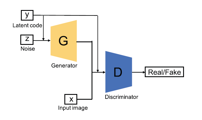
Conditional GAN (cGAN)
In this variant of GAN, both the generator and discriminator model are conditioned on some extra information $y$. Here $y$ can be class label or other modal data. The objective function of cGAN, therefore, becomes :
$\hspace{3em} \underset{G}{\min} \underset{D}{\max} V(D,G) = E_{x ∼ P_{\text{data}}(x)}[\text{log} D(x \mid y)] + E_{z∼ p_{z}(z)}[\text{log}(1-D(G(z \mid y)))]$
The key thing here is that $y$ is encoded inside the generator and discriminator before being concatenated with encoded $z$ and encoded $x$, this helps enhance cGAN discriminator ability to discriminate. Also, it helps cGAN handle multimodal datasets efficiently.
InfoGAN
InfoGAN proposed instead of using a single noise vector $z$, we can decompose it into two parts i.e, $z$ - the incompressible noise and $c$ - the latent code.
$c$ is used to target semantic structure on real data distribution. (Gui J. et al., 2021) The InfoGAN aims to solve :
$\hspace{3em} \underset{G}{\min} \underset{D}{\max} V_{I}(D,G) = V(D,G) - \lambda I (c;G(z,c))$
where,
$V(D,G)$ is the original objective function of GAN
$G(z,c)$ is the generated sample
$I$ is the mutual information
$\lambda$ is the tunable regularization parameter
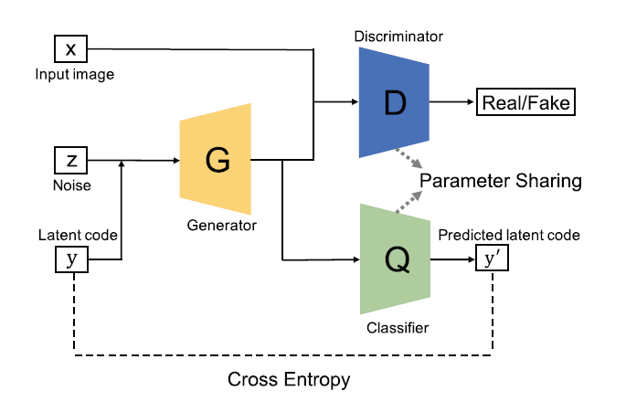
To make $c$ contain as much as meaningful features of the real samples as possbile, we need to maximize $I(c;G(z,c))$. However, to optimize $I(c;G(z,c))$ we need access to the posterior $P(c \lvert x)$ where $x$ is the real data distribution.
But, we can have a lower bound of $I(c;G(z,c))$ by defining a auxiliary distribution $Q(c \lvert x)$ to approximate $P(c \lvert x)$. The final objective function of InfoGAN, therefore, is :
$\hspace{3em} \underset{G}{\min} \underset{D}{\max}V_{I}(D,G) = V(D,G) - λ L_{I}(c;Q)$
where, $L_{I}(c;Q)$ is the lower bound of $I(c;G(z,c))$
Auxiliary Classifier GAN (AC-GAN)
AC-GAN contains an auxiliary classifier in its architecture, however it is similar to previously discussed cGAN and InfoGAN. In AC-GAN, each generated sample has a corresponding class label $c$ in addition to noise vector $z$, The important thing is here $c$ only refers to the class label unlike cGAN and InfoGAN where it can be domain data.(Wang et al., 2021)
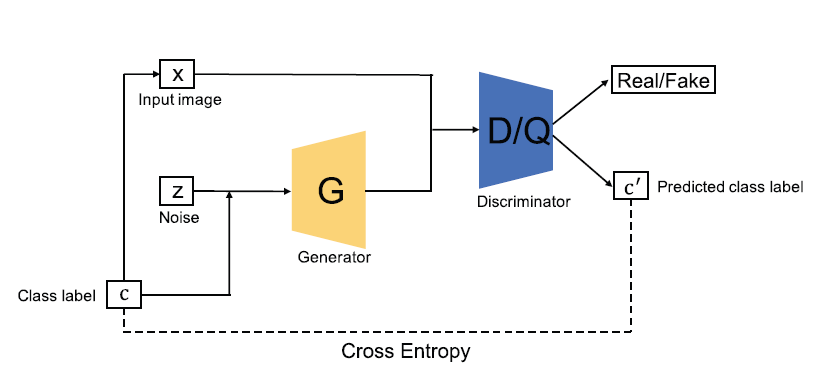
The discriminator in AC-GAN consists of a discriminator $D$ (distinguishes real and fake samples) and a classifier $Q$ (classifies real and fake samples), while sharing all weights except the last layer like InfoGAN. The loss function of AC-GAN can be constructed by considering the discriminator and classifier, as written below
`L_(S) = `𝔼`x~p_(r)``log[D(x | c)] + `𝔼`z~p_(z)``log[1-D(G(z | c))]`
`L_(C) = `𝔼`x~p_(r)``log[Q(x | c)] + `𝔼`z~p_(z)``log[Q(G(z | c))]`
where $D$ is trained to maximizing $L_{S} + L_{C}$ and $G$ is trained on maximizing $L_{C} - L_{S}$
Bi-Directional GAN (BiGAN)
BiGAN introduced the idea of learning from the inverse mapping i.e, by projecting data back into the latent space. The overall architecture of BiGAN consists of an Encoder $(E)$, a generator $(G)$ and a discriminator $(D)$.
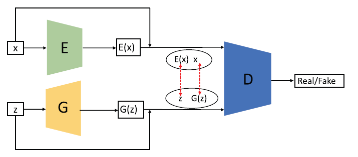
Here, $E$ encodes real sample data into $E(x)$ and $G$ decodes $z$ into $G(z)$, while $D$ aims to evaluate the difference between each pair of $(E(x),x)$ and $(G(z),z)$. The encoder and decoder must learn to invert one another to fool the discriminator.
LAPGAN
Laplacian Pyramid of Adversarial Networks (LAPGAN) is proposed to generate high resolution images from the lower-resolution input images. But let’s first understand the Laplacian Pyramid.
Laplacian Pyramid (LP) :
It is used to compact image representation, and consists of two basic steps :
- Convolve over the original image $I_{0}$ with a lowpass filter $v$ such as Gaussian filter and subsample it by 2 to create a reduced lowpass version of the image $I_{1}$
- Upsample $I_{1}$ by $u(\cdot)$ which inserts zeros in between each row and column and interpolating the missing values by convolving it with the same filter, $v$, to create an expanded lowpass image $u(I_{1})$ which then gets subtracted pixel-by-pixel from the original image $I_{0}$ to give the detail image - $h_{0}$ where $h_{0} = I_{0} - u(I_{1})$ (Pradham, Younan and King, 2008).
In order to compress now, $h_{0}$ and $I_{1}$ are encoded, because firstly, $I_{1}$ is the lowpass version of the original image, and $h_{0}$ is largely decorrelated.
This step then gets performed recursively on the lowpass and subsampled image $I_{1}$ a maximum number of $k$ times if the original image is of $2^k × 2^k$. This process then provides a number of detail images $h_{0},h_{1},\cdots,h_{k}$ and the lowpass image $I_{k}$.
$\hspace{3em} h_{k} = I_{k} - u(I_{k+1})$
These recursively obtained image in the series is smaller in size by a factor of four compared to the previous image and its center frequency reduced by an octave.
We, however with inverse transform or recurrence can obtain the original image, $I_{0}$ from the $k$ detail images $h_{0}, h_{1}…,h_{k}$ and the lowpass image $I_{k}$ with following steps :
-
$I_{k}$ is upsampled by $u(\cdot)$ which inserts zeros between the sample values and interpolating the missing values by convolving it with the filter $v$ to obtain the image $u(I_{k})$
-
The image $u(I)$ is added to the lowest level detail image $h_{k}$ to obtain the approximation image at the next upper level:
$\hspace{3em} I_{k} = h_{k} + u(I_{k+1})\qquad\qquad..eq(1)$
- Step 1 and step 2 are repeated on the detailed images $h_{0},h_{1},\cdots,h_{k-1}$ to obtain the original image.
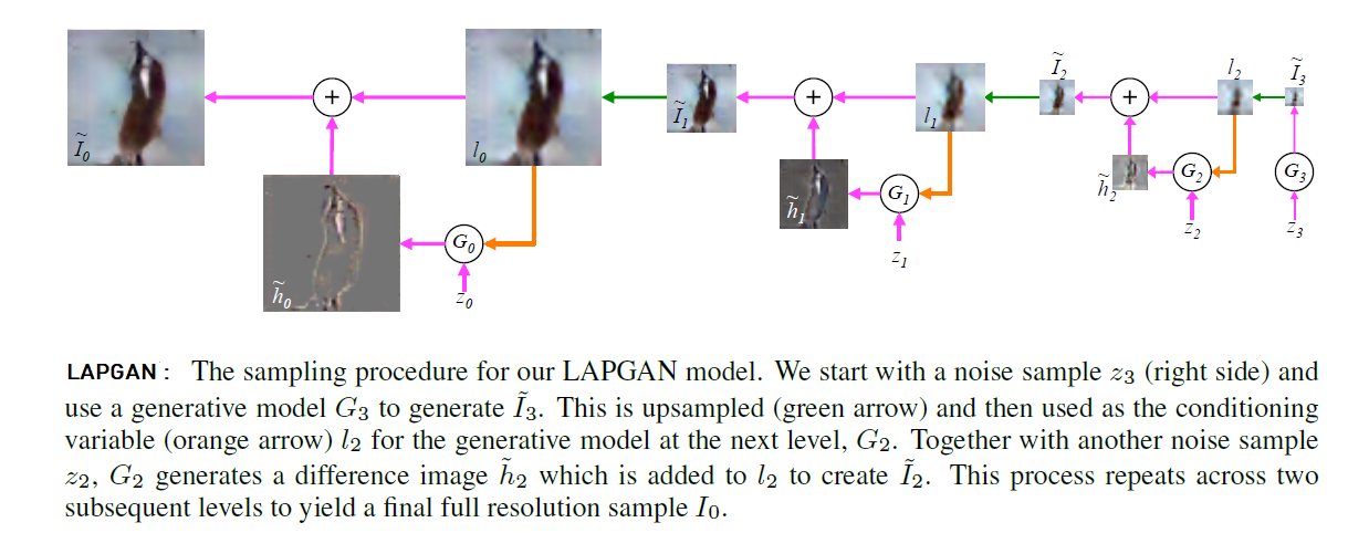
LAPGAN Architecture
LAPGAN combines conditional GAN (cGAN) with Laplacian Pyramid representation with a sampling procedure. Here, we first generate a set of generative convnet models i.e,$[G_{0},\cdots,G_{k}]$.
Each of these ConvNet models then captures the distribution of coefficients $h_{k}$ for natural images at a different level of the Laplacian Pyramid. This is the sampling procedure earlier mentioned, and it is similar to inverse transform as in eq(1), except that the generative models are used here to produce $h_{k}$
However, at each level of Laplacian Pyramid, these $h_{k}$ are produced with stochastic choices (with equal probability) to either construct the $h_{k}$ using standard procedure or generate them using $G_{k}$
$\hspace{3em} \tilde{h_{k}} = G_{k}(z_{k},u(I_{k+1}))$
Then, eq(1) can be re-written as :
$\hspace{3em} \tilde{I_{k}} = \tilde{h_{k}} + u(\tilde{I_{k+1}})$
$\hspace{5em} = G_{k}(z_{k} u(I_{k+1})) + u(\tilde{I_{k+1}})$
Recurrence starts by setting $\tilde{I_{k+1}} = 0$ and using the model at the final level $G_{k}$ to generate a residual image $\tilde{I_{k}}$ using noise vector $z_{k}$, and it is repeated at all levels except the final.
The key thing to note here, is $G_{k}$ is just the generative part of GAN here, we use $D_{k}$ for discriminator that takes $h_{k}$ or $\tilde{h_{k}}$ along with the lowpass image $I_{k}$, explicitly added before the first convolutional layer, to predict if the image was real or generated.
References :
- Goodfellow, I., Pouget-Abadie, J., Mirza, M., Xu, B., Warde-Farley, D., Ozair, S., Courville, A. and Bengio, Y., 2014. Generative adversarial nets. Advances in neural information processing systems, 27.
- Gui, J., Sun, Z., Wen, Y., Tao, D. and Ye, J., 2021. A review on generative adversarial networks: Algorithms, theory, and applications.IEEE Transactions on Knowledge and Data Engineering.
- Wang, Z., She, Q. and Ward, T.E., 2021. Generative adversarial networks in computer vision: A survey and taxonomy. ACM Computing Surveys (CSUR), 54(2) pp.1-38.
- Pradham, P., Younan, N. and King, R., 2008. Concepts of image fusion in remote sensing applications. Image Fusion, pp.393-428