YOLO
You Only Look Once (YOLO) is a single convolutional neural network based model, which unlike,R-CNN based models, simultaneously, predicts multiple bounding boxes and its class probabilities of those boxes (Redmon et al., 2016). A few advantages of YOLO are:
- YOLO is extremely fast. As frame detection doesn’t go into a complex pipeline, but taken as a regression problem, YOLO gets to process streaming video real-time with less than 25 milliseconds of latency.
- It, unlike sliding window and Region-proposal based technique, uses feature extracted from the entire image, to predict all bounding boxes and its classes.
- YOLO, also, gets to generalize well with unexpected input images/frames - just lags a bit with accuracy.
Detection
YOLO system divides the input image into an \(S × S\) grid, where each grid cells preditcs \(B\) bounding boxes.
Each bounding boxes consists of 5 predictions i.e, \(x, y, w, h\) and confidence, where \((x,y)\) represent the center of box relative to grid cell. \((w,h)\) relative to the whole image.
Confidence is given by \(Pr(Object) ∗ IOU_{pred}^{truth}\) and represent confidence of box containing object and its accuracy.
Each grid cell also predicts \(C\) class probabilities \(Pr(Class_{i} \mid Object)\) This is probability of grid containing an object - it predict one class probability per grid cell.
At test time, both class probabilities gets multiplied \(Pr(Class_{i} \mid Object) ∗ Pr(Object) \ast IOU_{pred}^{truth}\), providing information on probability of object class in the box, and how well box fits the object.
Network Architecture
Architecture of YOLO is inspired by googLeNet. It has 24 convolutional layers, followed by 2 Fully-connected layers, and instead of inception blocks used in googLeNet, YOLO use \(1 × 1\) reduction layer - to reduce the feature space from preceding layers, followed by \(3 × 3\) convolutional layer. Network architecture is as shown below:
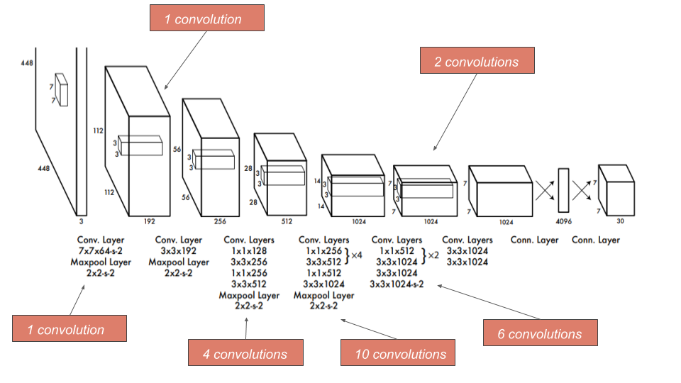
During training \(224 × 224\) resolution image is used, however during detection, \(448 × 448\) reolution is used for fine-grained visual information. Similarly, linear activation function is used in the final layer, whereas leaky ReLU is used in all the layers prior to it.
Loss Function
As YOLO detection consists of three phases: 1. detecting bounding box 2. Confidence of box (containing object and its accuracy), and 3. Class probability. Loss Function of YOLO is also have three distinct parts:
Localization Loss
In this, as sum-squared error weights error in small and large boxes equally, it can fail to converge quickly, as small deviations in large bouding boxes matter less than small deviations in small bounding boxes. It is addressed by simply using square-root of height and width. Localization Loss can be stated as:
\[\text{Localization Loss} = \lambda_{coord} \sum\limits_{i=0}^{S^2} \sum\limits_{j=0}^{B} 1_{ij}^{obj} \left[(x_{ij} - x_{ij}^{gdt})^2 + \left(y_{ij} - y_{ij}^{gdt}\right)^2 + \left(\sqrt{w_{ij}} - \sqrt{w_{ij}^{gdt}}\right)^2 + \left(\sqrt{h_{ij}} - \sqrt{h_{ij}^{gdt}}\right)^2\right]\]where,
\(S^{2}\) is the number of grid cells, \(B\) is the number of bounding boxes per grid cell, \(\lambda_{coord}\) is the coefficient to scale the localization loss, and \(1_{i}^{obj}\) is the indicator function that equals \(1\) if the \(i^{th}\) grid cell in the \(j^{th}\) bounding box contains an object.
Confidence Loss
It measures the discrepancy between predicted confidence score (of having object in the box) and ground-truth score. However, as grid in the image, may not any object. It can push confidence score of cell to zero. To remedy this, we increase the loss from bounding box coordinate predictions and decrease the loss from confidence predictions for boxes that don’t contain objects, using two parameters i.e, \(\lambda_{coord}\) and \(\lambda_{noobj}\), with values \(5\) and \(0.5\) respectively. If \(C\) is the predicted confidence, and \(C^{gdt}\) is ground-truth confidence, then Confidence Loss then can be expressed as:
\[\text{Confidence Loss} = \lambda_{coord} \sum\limits_{i=0}^{S^2} \sum\limits_{j=0}^B 1_{ij}^{obj} \left(C_{ij} - C_{ij}^{gdt}\right)^2 + \lambda_{noobj} \sum\limits_{i=0}^{S^2} \sum\limits_{j=0}^B 1_{ij}^{noobj} \left(C_{ij} - C_{ij}^{gdt}\right)^2\]Classification Loss
It measures the discrepancy between the predicted class probabilities and the ground truth class labels. It is also computer using cross-entropy, and if \(p_{i}\) is predicted class probability, with \(p^{gdt}\) as ground-truth class labels, we can write classification loss as :
\[\text{Classification Loss} = \sum\limits_{i=0}^{S^2} 1_i^{obj} \sum_{c ∈ classes} (p_{i}(c) - (p_{i}^{gdt}(c))^2)\]Total Loss, thereafter, is the sum of all three losses, i.e, \(\text{Total Loss} = \text{Localization Loss} + \text{Confidence Loss} + \text{Classification Loss}\)
which then gets used to updated weights of YOLO architecture through backpropagation. YOLO architecture, however, have a few limitations such as being Prone to Localization Error.
Retina Net
Focal Loss
Focal Loss is designed to address the class imbalance problem, where the number of background (non-object) samples greatly outweighs the number of object samples.
Focal Loss is based on cross-entroy loss, but designed to down-weight easy (well-classified) examples, and focussing on hard negatives (misclassified) examples during training. It adds a modulating factor \((1 - p_{t})^\gamma\) to cross-entroy, and tunable parameter \(γ \gt 0\), and Focal Loss can be stated as:
\[FL(p_{t}) = -(1 - p_{t})^{γ} log(p_{t})\]where, \(p_{t}\) is the predicted probability of the true class label.
Here, when an example is misclassified and \(p_{t}\) is small, the modulating factor is near \(1\) and almost equivalent to cross-entropy. On the other hand, if \(p_{t}\) is large i.e, \(p_{t} → 1\), the modulating factor goes to \(0\), and loss for well-classified example is down-weighted.
However, for practical purposes, we add a balancing factor \(\alpha_{t}\) to Focal Loss, making it :
\[FL(p_{t}) = - \alpha_{t}(1 - p_{t})^{\gamma}\log(p_{t})\]\(\alpha_{t}\) ,as a balancing factor, adjusts the weight of positive (presence of object) and negative (non-bject) examples in the loss. Specifically, \(\alpha\) represents the weight assigned to the positive examples relative to the negative examples.
By default, \(\alpha\) is set to \(0.25\), which means that positive examples (anchorboxes with object) have a weight of \(0.25\), while negative examples (anchorboxes with non-objects) have a weight of \(1 - α = 0.75\)
Retina Net Architecture
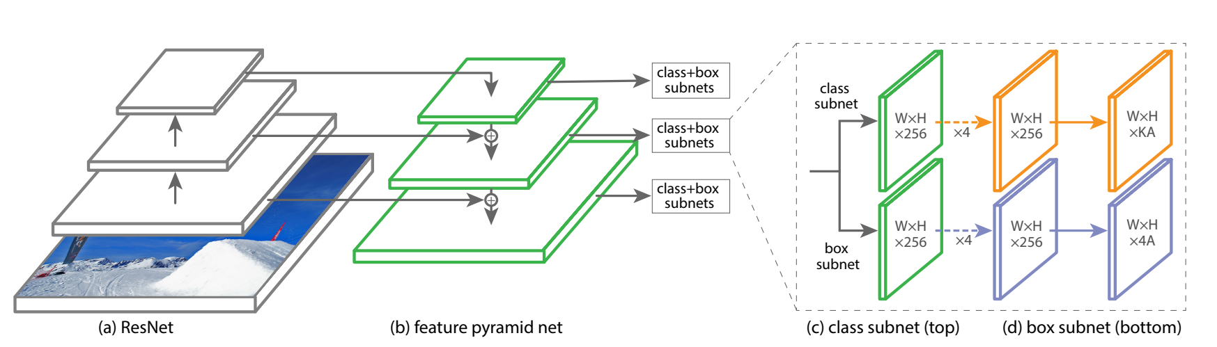
Architecture of Retina Net is composed of one backbone network that is responsible for computing a convolutional feature map over the entire image, and two task-specific subnets. The first is Classification Subnet performing convolutional object classification on the backbone’s output, and the second is Box Regression Subnet performs convolutional bounding box regression.
Single Shot Detector (SSD)
References
- Redmon, J., Divvala, S., Girshick, R. and Farhadi, A., 2016. You only look once: Unified, real-time object detection. In Proceedings of the IEEE conference on computer vision and pattern recognition(pp. 779-788).
- Lin, T.Y., Goyal, P., Girshick, R., He, K. and Dollár, P., 2017. Focal loss for dense object detection. In Proceedings of the IEEE international conference on computer vision(pp. 2980-2988).
- Lin, T.Y., Dollár, P., Girshick, R., He, K., Hariharan, B. and Belongie, S., 2017. Feature pyramid networks for object detection. In Proceedings of the IEEE conference on computer vision and pattern recognition (pp. 2117-2125).