Population: Population is a set of similar items or events that is of interest for some statistical problem. It can be a group of existing object or a hypothetical or potentially infinite group of items.
Sample: Sample is a selection of individual, events or objects taken from a well-defined population. Thus sample is a subset of population.
Parameters: These are those quantities that summarizes or describes an aspect of the population such as mean, deviation, correlation, etc.
Sampling Error: It is the difference between sample statistics and population parameters. Since, samples does not include all elements of population, its estimate tends to differ from it.
Range :Range is the difference between the smallest and the largest data value.
Quartiles, Deciles, Percentiles: Quartiles divide a set of observations into 4 equal parts. Deciles divide them into 10 equal parts, whereas Percentiles divide observations into 100 equal parts.
Mode : Mode is the score that occurs most often in a frequency distribution of data.
Median : Median is the middle score found by arranging a set of numbers from the smallest to the largest (or from largest to smallest). If even number in data point, then median is the average of two middle values.
Mean : Mean is the arithmetic average of numbers in a data set i.e, sum of numbers divided by the total.
Geometric Mean: Geometric mean (GM) is the average change of percentage, ratios, indexes or growth rate over time. If we have a set of n positive numbers, then its GM is defined as the nth root of the product of n values.
It can also be used to get Rate of Increase Over Time. In this case, GM is calculated as:
\[\text{GM} = \sqrt[n]{\frac{\text{Value at the end of period}}{\text{Value at start of period}}} -1\]Harmonic Mean : Harmonic Mean(HM) is the reciprocal of the arithmetic mean, and useful when averages of ratios, and rates are needed. If we have a set of $n$ numbers, then its HM is defined as:
\[HM = \frac{n}{\frac{1}{x_{1}} + \frac{1}{x_{2}} + \cdots + \frac{1}{x_{n}}}\]Expected Value
Expected value is the weighted average of a random variable according to the probability distribution. It is supposed to be the approximate measure of center of a distribution. Simply put, if we have random variable $X$ with finite list of $x_1, x_2 \cdots x_n$ with probability of occurence as $p_1, p_2 \cdots p_n$, then the Expected Value of X or $E[X] = x_{1}p_1, x_{2}p_2, \cdots x_{n}p_n$
So, the Expected value of a random variable $X$ can be represented as:
Note: If $X$ is a randon variable, and $a$, $b$ and $c$ are some constants, then for any functions $g_1(x)$ and $g_2(x)$ whose expectations exists:
- $E(ag_{1}(X) + bg_{1}(X) + c) = aEg_{1}(X) + bEg_{1}(X) + c$
- if $g_{1}(X) \ge 0$ for all x, then $Eg_{1}(X)\ge0$
- If $g_1(X) \ge g_2(X)$ for all $x$, then $Eg_{1}(X) \ge Eg_{2}(X)$
- If $a \le g_1(X) \le b$ for all $x$, then $a \le Eg_1(X) \le b$
**Moments
We know that first moment is mean($\mu$), second moment is variance. Also,standardized moment is $\frac{\text{Moment}}{\sigma^n}$. We also know that first standardized moment is 0, and second is 1. Second being 1 makes sense as $\frac{var(X)}{\sigma^2}$ will be 1, but first standardized moment does not as $\frac{\mu}{\sigma}≠ 0$. In most books, it is not covered, and wherever it is (including wikipedia), it is mentioned as (raw) first moment is mean, $\mu$ and second central moment is variance. Casella & Berger said it is n-th moment of $X$ : $\mu_{n} = EX^n$ and n-th central moment of $X$: $\mu_{n} = E(X - \mu)^n$.
So, there must be two first moment - $1$. raw first moment i.e, Expected value ($EX$) or Mean, $\mu$, and $2$. first central moment i.e., $0$ because $E(X - \mu)^1 = 0$, measuring spread from Expected Value or Mean to mean.
Variance
Variance is the second central moment of a random variable $X$ and can be given by $E(X - \mu)^2$.
We can write it as:
Key things:
- From $\text{Var}(X) = E[(X - EX)^2]$, we can further derive that: $\text{Var}(X) = E[X^2] - E[X]^2$
- Variance of a constant is zero i.e, $\text{Var} (a) = 0$
- $\text{Var} (X + a) = \text{Var} (X)$
- $\text{Var}(aX + b) = a^2 \text{Var}X$
Standard Deviation
Standard deviation ($\sigma$) is square root of variance, and is a good measure for having same unit as data, to ascertain if most values are closer to the expected value (by having lower $\sigma$) or farther away by having larger $\sigma$. We can define it as:
\[σ = \sqrt{E[(X - \mu)^2]} \quad \text{or} \qquad\sqrt{\int_{-\infty}^{\infty}(x - \mu)^2 f(x)dx}\]It can further be written as: $\sqrt{E[X^2] - E[X]^2}$
Standardized Moment
It is used to make moment scale-invariant. The standardized moment of degree $k$ normalizes central moment of degree $k$ by standard deviation $\sigma^k$.
- First central moment is $0$. Therefore, first standardized moment i.e, $\frac{0}{\sigma^1} = 0$
- Second central moment is variance. Therefore, second standardized moment is given as: $\frac{\text{Variance}}{\sigma^2} = \frac{E[(X - \mu)^2]}{(\sqrt{E[(X - \mu)^2]})^2} = 1$.
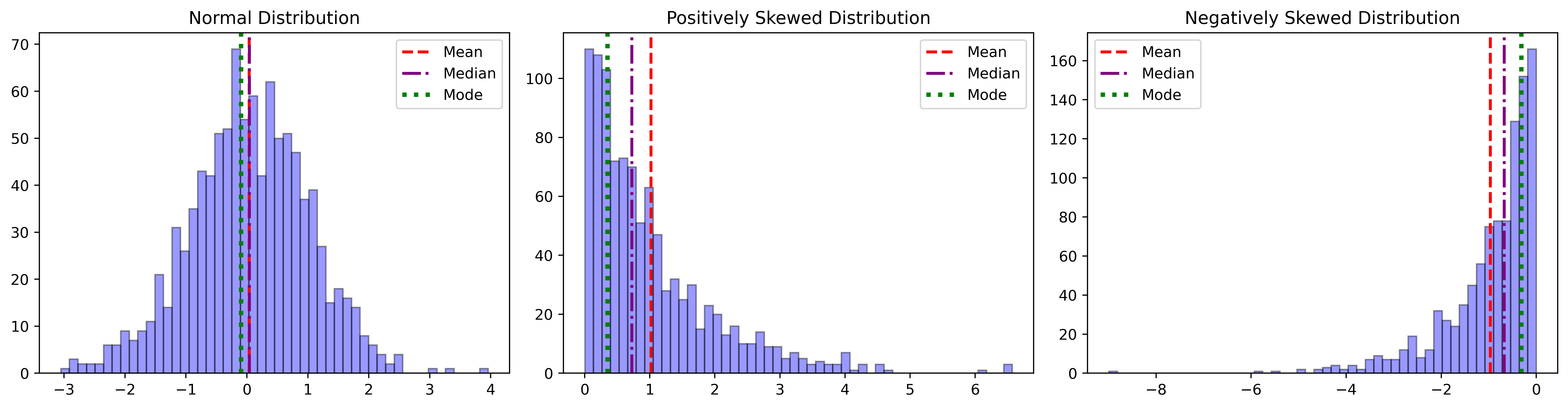
Skewness
Skewness is the third standardized moment and therefore can be given by:
\[\tilde{μ_3} = \frac{E[(X - \mu)^3]}{\sigma^3}\]Expanding eq($8$), we can further derive it as: $\tilde{μ_3} = \frac{E[X^3] -3μ σ^2 - μ^3}{\sigma^3}$. Also, if we know value of Mode and Median of our data, simpler calculation can be made by:
- Pearson first skewness coefficient i.e, $\frac{\text{Mean} - \text{Mode}}{\text{std. dev.}}$
- Pearson second skewness coefficient i.e, $\frac{3\cdot (\text{Mean} - \text{Median})}{\text{std. dev.}}$
In general, if Mean $\gt$ Mode, it is said to be positively skewed for having long tail on the right side, and if Mean $\lt$ Mode, it is negatively skewed for having tail on the left side of the distribution.
Kurtosis
Kurtosis $\kappa$ is the fourth standardized moment and can be given by:
\[\tilde{μ_4} = \frac{E[(X - \mu)^4]}{\sigma^4}\]Kurtosis is bounded below at lower limit of squared skewness + $1$ i.e, $\frac{\mu_{r}}{\sigma_{4}} \ge (\frac{\mu_{3}}{\sigma_{3}})^2 + 1$. It, however, does not have upper bound.
For a normal distribution, we have kurtosis, $\kappa =3$. We derive a term Excess Kurtosis, $\kappa’$ from here i.e. $\kappa’ = \kappa - 3$.
- If $\kappa’ = 0$, we have normal distribution, and called Mesokurtic
- If $\kappa’ \gt 0$, we have sharp peak, and heavy tail in distribution. It is called Leptokurtic.
- if $\kappa’ \lt 0$, we have flat peak, and light tail in distribution. It is called platykurtic.
*Z-score
Z-Score (or Standard Score) is a measure to describe how far is the data from the mean. It is standardizing the data by transforming it into a normal distribution with mean at $0$ and standard deviation of $1$. It can be done by:
\[\text{Z-Score} = \frac{X - \mu}{\sigma}\]- A positive Z-Score means $X$ is above $\mu$
- A negative Z-Score means $X$ is below $\mu$
- A Z-Score of $0$ means $X = μ$, and data point above or below $(+/-)3$ are considered outliers.
Bi-Variate Concepts
Joint Distribution
Marginal Distribution
Covariance
Covariance is the measure of how two random variables are related, if we have $X$ and $Y$ as random variable, covariance is given by:
\[\text{Cov}(X,Y) = E((X - \mu_{X})(Y - \mu_{Y}))\]- If large values of $X$ tends to be observerd with large values of $Y$, and small values of $X$ with the small values of $Y$, then $\text{Cov}(X,Y)$ will be positive.
- If large values of $X$ tend to be observed with small values of $Y$, and small values of $X$ with the large values of $Y$, then $\text{Cov}(X,Y)$ will be negative.
Important Theorems:
-
For any two random variable $X$, and $Y$, \(\text{Cov}(X,y) = EXY - \mu_{X}\mu_{Y}\)
-
If $X$ and $Y$ are independent random variables then, $\text{Cov}(X,Y) = 0$. It does not mean if $\text{Cov}(X,Y) = 0$, then $X$ and $Y$ are independent.
-
If $X$ and $Y$ are two random variables, and $a$ and $b$ are any two constants, then
Correlation
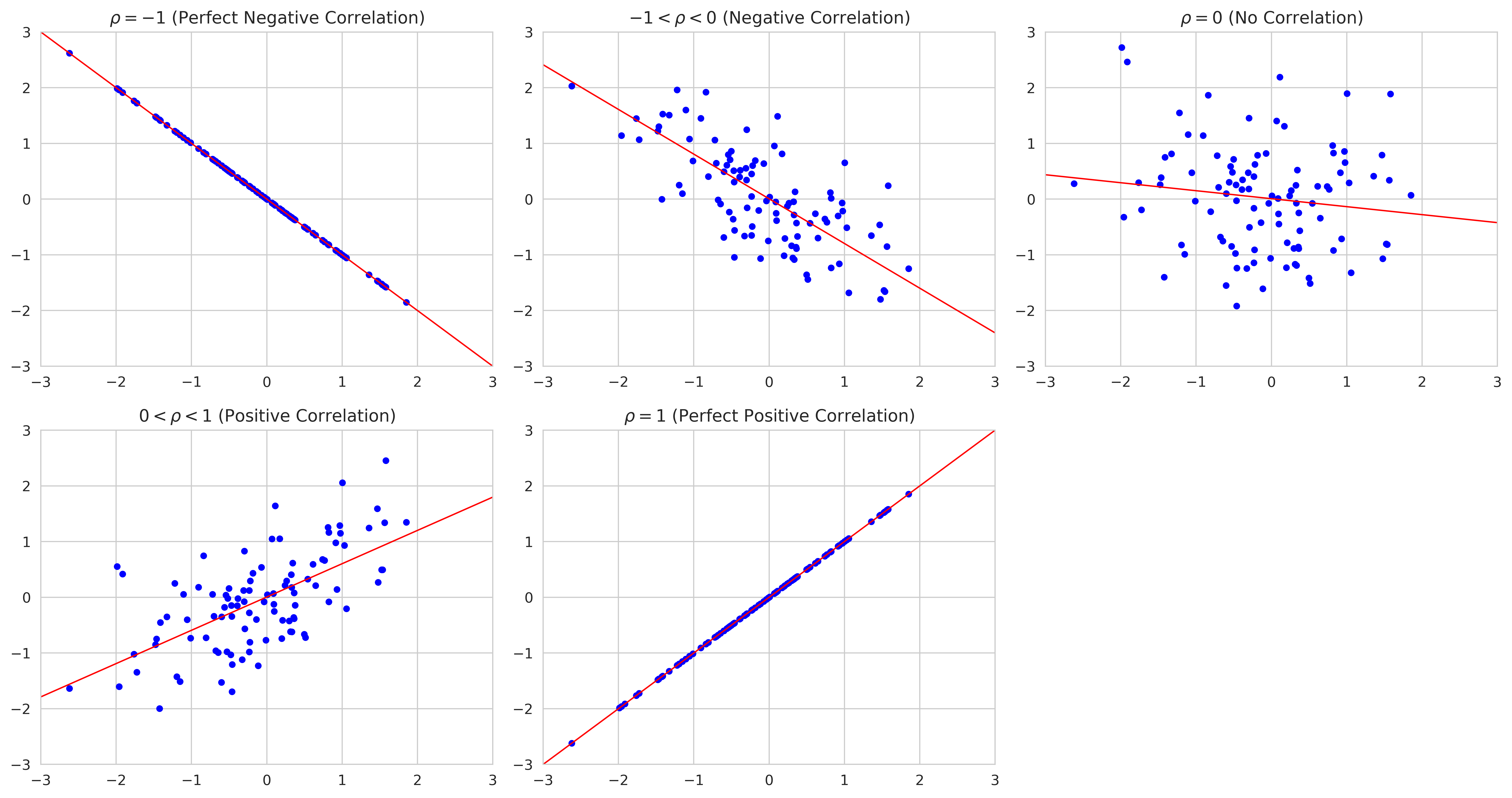
Correlation is another measure to provide information on the relationship between any two random variable, $X$ and $Y$. As it is bounded between $-1$ and $1$, we get to know the strength of relationship between $X$ and $Y$. It is defined as :
\[\rho_{XY} = \frac{\text{Cov}(X,Y)}{\sigma_{X}\sigma_{Y}}\]- If $X$ and $Y$ are independent randon variable, then $\rho_{XY} = 0$.
- $-1 \le \rho_{XY} \le 1$
- If $\rho_{XY}$ is negative, $X$ and $Y$ are inversely correlated, and if $\rho_{XY}$ is positive, $X$ and $Y$ are strongly correlated. This is illustrated below:
Pearson Correlation Coefficient
Pearson Correlation Coefficient (PCC) is same as correlation coefficient $\rho_{XY}$ mentioned in eq$(13)$. However, it is specifically suitable when we have random variable $X$ and $Y$ linearly related, and normally distributed.
For population, eq($13$) is perfect. For sample, we can write PCC as:
\[\text(PCC) = \frac{\sum_{i=1}^n (X_{i} - \mu_{X})(Y_{i} - \mu_{Y})}{\sqrt{\sum_{i=1}^n(X_{i} - \mu_{X})^2(Y_{i} - \mu_{Y})^2}}\]Spearman’s Rank Correlation Coefficient
Spearman’s Rank Correlation Coefficient (SRCC) is more robust. It works with ordinal data, data that are normally distributed and have outliers. It is suitable with non-linear relationship between variables as well. This is achieved by the introduction of fractional ranking and mean centering.
Fractional Ranking: In this, we sort the data first in ascending order assigning lowest rank to the first value. When we encounter two or more consecutive ranks with same values, we take mean of their ranks, and assign mean-rank to all values.
Mean Centering: At first, we find the mean-center for all $N$ values by $\frac{N+1}{2}$. Then, we substract every rank in our data by mean-center to get our mean centered data.
Spearman’s Rank Correlation is represented by $r_{s}$ and constrained as $-1 \le r_{s} \le 1$.
- $r_{s} = 1$ means monotonic increasing relationship between $X$ and $Y$
- $r_{s} = -1$ means monotonic decreasing relationship between $X$ and $Y$
- $r_{s} = 0$ means linear relationship between $X$ and $Y$
For sample, after fractional ranking and mean centering, our spearman’s rank coefficient, $r_{s}$ is given by:
\[r_{s} = \frac{\sum_{i=1}^n (RX_{i} - R\mu_{X})(RY_{i} - R\mu_{Y})}{\sqrt{\sum_{i=1}^n(RX_{i} - R\mu_{X})^2(RY_{i} - R\mu_{Y})^2}}\]If all $n$ ranks are distinct integers, it can be computed as:
\[r_{s} = 1 - \frac{6 ∑ d_{i}^2}{n(n^2 - 1)}\]where \(d_{i} = R(X_{i}) - R(Y_{i})\) is the difference between the two ranks of each obsevation, and \(n\) is the number of observations.
Inequalities
Lemma: If $a$ and $b$ are any positive numbers, and $p$ and $q$ are any positive numbers (necessarily greater than $1$) satisfying $\frac{1}{p} + \frac{1}{q} =1$, then :
\[\frac{1}{p}a^p + \frac{1}{q}b^q \ge ab\]Holder’s Inequality
Let $X$ and $Y$ be any two random variables, and let $q$ and $q$ satisfying lemma (17). Then,
\[\lvert EXY \rvert \le E\lvert XY \rvert \le (E\lvert X \rvert^p)^{\frac{1}{p}}(E\lvert X \rvert^q)^{\frac{1}{q}}\]Cauchy-Swartz Inequality
This is a special case of Holder’s Inequality for which $p = q = 2$. Let define it as: For any two random variables, $X$ and $Y$,we have:
\[\lvert EXY \rvert \le E\lvert XY \rvert \le (E\lvert X \rvert^2)^{\frac{1}{2}}(E\lvert X \rvert^2)^{\frac{1}{2}}\]- If $X$ and $Y$ have means $\mu_X$ and $\mu_Y$ and variance $σ^2_X$ and $σ^2_Y$, respectively, we can apply Cauchy-Swartz Inequality to get:
- And squaring both side in $(20)$ and using statistical notations, we can also get:
Minkowski’s Inequality
Let $X$ and $Y$ are any two random variables. Then for $1 \le p \le \infty$, we have:
\[[E\lvert X+Y \rvert^p]^{\frac{1}{p}} \le [E\lvert X \rvert^p]^{\frac{1}{p}} + [E\lvert Y \rvert^p]^{\frac{1}{p}}\]Jensen Inequality
For any random variable, $X$, if $g(x)$ is a convex function, then $Eg(X) \ge g(EX)$.
Equality holds if and only if, for every line $a+bx$ that is tangent to $g(x)$ at $x = EX$, $P(g(X) = a+ bX) =1$
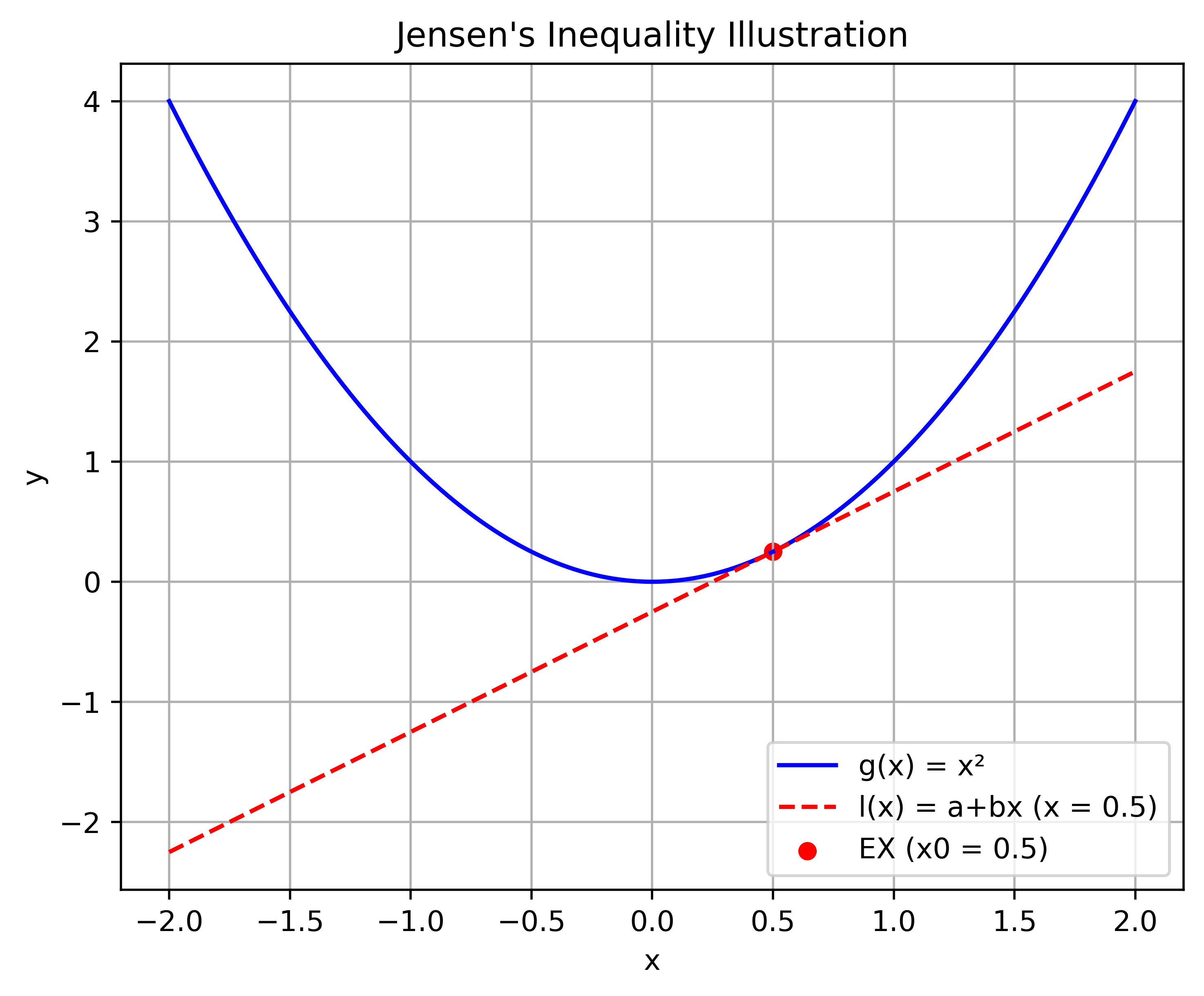
- One application of Jensen’s inequality shows that $EX^2 \ge (EX)^2$ since $g(x) = x^2$ is convex.
- Also, if $x$ is positive, then $\frac{1}{x}$ is convex, hence $E(\frac{1}{X}) \ge \frac{1}{EX}$.
- The function of $g(x)$ is convex if $g^{‘’}(x) \ge 0$ for all $x$
- The function of $g(x)$ is concave if $g^{‘’}(x) \le 0$ for all $x$. And if $g(x)$ is concave, we have $Eg(X) \le g(EX)$.
Reference
- Casella, G. and Berger, R., 2024. Statistical inference. CRC press.
- Lind, D.A., Marchal, W.G. and Wathen, S.A. (2023) Statistical techniques in business and Economics. 17th edn. McGraw-Hill Education.