Point Processes are those processes where each output pixel value depends on only the corresponding input pixel values. It can be pixel transform, color and brightness correction or other transformations.
Pixel Transformer
A general pixel transformer is a function that takes one or more input images and produces an output image. It can be defined as:
$\hspace{3em} g(X) = h(f(X))\,$ or $\, g(X) = h(f_{0}(X), … ,f_{n}(X))$
where $X$ is D-dimensional (usually $D=2$ for images). For discrete images, the domain consists of a finite number of pixel location, $x = (i,j)$. The above equation can be written as :
$\hspace{3em} g(i,j) = h(f(i,j))$
However, two commonly used point processes with image are multiplication and addition with a constant. i.e,
$\hspace{3em} g(X) = a f(X) + b$
where parameters, $a \ge 0$ and $b$ are called gain and bias parameters that control contrast and brightness respectively. We know that bias and gain can also be spatially varying, therefore, $g(X)$ can be written as :
$\hspace{3em} g(X) = a(X)f(X) + b(X)$
- Linear Blend : It is another common operator and is used to perform a temporal cross-dissolve between two images or videos by varying $\alpha$ from $0 \to 1$ in the given equation below:
$\hspace{3em} g(X) = (1 - \alpha)f_{0}(X) + \alpha f_{1}(X)$
- Gamma Correction : This highly used non-linear transform is used to remove the non-linear mapping between input raidnace nd qunatizex pixel values. To invert the gamma mapping applied by the sensor, we use :
$\hspace{3em} g(X) = [f(X)]^{1/γ}$
where a gamma value of $γ \approx 2.2$ is a reasonable fit.
Compositing and Matting
Matting : In photo/video applications, when an object need to cut out from place and put it on top of another, matting is the process of extracting the object from the original image.
Compositing : It is process inserting an object into another image.
The intermediate representation used for the foreground object between these two stages is called an alpha-matted color image. This alpha-matted color image contains a fourth alpha channel $\alpha$ making channel RGBA. It describes the relative amount of opacity at each pixel.
Pixels within the oject are fully opaque $(\alpha = 1)$, while pixels fully outside the object are transparent $(\alpha = 0)$. Pixels on the boundary vary smoothly between these two extremes.
To Composite a new (or foreground) image op top of an old image, the over operator is used :
$\hspace{3em} C = (1 - \alpha)B + α F$
This operator attentuates the influence of the background image, $B$ by a factor of $(1 - \alpha)$ and then in the color (and opacity) values corresponding to foreground image, $F$
Histogram Equalization
Making Histogram of an image is to plot the individual color channels and luminance values within the image. From Histogram, we can compute relevant statistics lik maximum, minimum, and average intensity values.
If we need to improve brightness and gain control of an image in a way that automatically determines their best value, we need to have flat Histogram.
Histogram Equalization is the way to do it, it helps to find an intensity mapping function $f(I)$ such that the resulting histogram is flat. The trick to finding such a mapping function is to first compute the Cumulative Distribution Function (CDF) $c(I)$.
$\hspace{3em} c(I) = \frac{1}{N} \sum_{i=0}^{I} h(i) = c(I - 1) + \frac{1}{N} h(I)$
where $N$ is the number of pixels in the image, when working with 8-bit pixel values, the $I$ and $c$ axes are rescaled from $[0,255]$, and $c(I)$ helps determine the final value that the pixel should take when histogram is flat by applying $f(I) = c(I)$.
However, the resulting image, then, lacks contrast, and muddy-looking which can be compensated by applying mapping function as :
$\hspace{3em} f(I) = α c(I) + (1-α )I$
Adaptive Histogram Equalization
If the pixel intensity varies a lot throughout the image, making certain region of image significantly darker or lighter than the most of the image, it is preferable to divide the image into $M × M$ block and perform seprate histogram equalization in each sub-block.
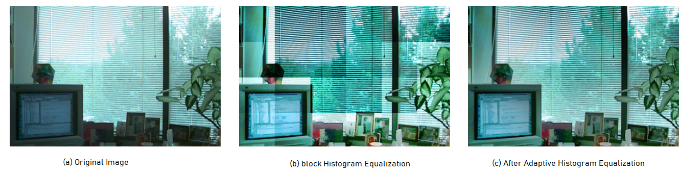
However, this kind of equalization can give rise to the visualization of sub-block borders as shown in the image above, and fails to sup1ress noise in b1ckground To overcome this, a bilinear interpolation is carried out with below given mapping:
$\hspace{3em} y = T(x) = round (\frac{L_{max}-1}{N × M}H_{c}k) \quad 0 \le x \lt L_{max}$
where $y=T(x)$ is transformation function, $N × M$ is input image, $L_{max}$ is maximum gray level, $H_{c}$ cumulative histogram
CLAHE
Contrastive Limited Adaptive Histogram Equalization (CLAHE) solves the noise problem, by limiting the improvement of the contrast. The slope associated with the gray level assignment gets limited by cutting 1 contrast factor the local histogram over a certain value.
With a low factor, the maximum slope of the local histogram will be low resulting in poor improvement. For example, contrast factor value of 1 keeps it at original image value essentially, whereas high factor such as $100$ makes it AHE.
Therefore, we set a $\beta$ threshold called clip limit for which the histogram will be cut at that value. This value is linked to a cut factor $\alpha$ (clip factor) in percentage as follows:
$\hspace{3em} \beta = \frac{N × M}{L_{max}}(1 + \frac{\alpha}{100}(s_{max}-1))$
where $S_{max}$ is the maximum possible slope value, and as $\alpha$ values varies between $0$ and $100$, maximum slope gets decided.
Numerical Spatial Filtering
Principle of Superimposition : If the input to the system consists of a weighted sum of different images, the system’s response is the Superimposition (that is weighted sum) of the responses to the individual input images.
Linearity : For example, If $I_{1}(i,j)$ and $I_{2}(i,j)$ are two images with $a$ and $b$ arbitary constants, and $\Theta$ represents an operator that transforms an image into another with the same dimensions, then it can be said that operator $\Theta$ is linear, if and only if it follows the Principle of Superimposition.
$\hspace{3em} \Theta\left[a ⋅ I_{1}(i,j) + b ⋅ I_{2}(i,j)\right] = a \cdot {I_{1}(i,j)} + b ⋅ \Theta\left[I_{2(i,j)}\right]$
Homogeneity Property : By multiplying the input image $I_{1}$ by a constant $\alpha$, the linear system responds with the appropriate value corresponding to the input image multiplied by the same constant $\alpha$.
$\hspace{3em}\Theta\left[α ⋅ I_{1}(i,j)\right] = \alpha ⋅ \Theta\left[I_{1h1(i,j)}\right]$
Impulse Response and Point Spread Function :
Following Superimposition principle, we can derive the nature of operator applied to an image just by observing only the output image. This is achieved as follow :
1. Decomposing the input image `I(i,j)` into elementary components
2. Evaluate the system's response to each elementary components.
3. Calculate the overall system reponse for the desired input by simply adding the individual outputs.
Appropriate tool for image decomposition is Dirac Delta Function, using this, the image `I(i,j)` is defined as a linear combination of translated delta functions
`I(i,j) = \sum_{l=0}^(N-1)\sum_{k=0}^(M-1) I(l,k) ⋅δ(i-l,j-k)` ...eq(1)
`= \sum_{l=0}^(N-1)\sum_{k=0}^(M-1) I(l,k) ⋅δ(i,j;l,k)`
where, if `δ(l,k) = 0 l≠0, k≠0` and if `δ(l,k) = 1 l = k = 0`
Also, `I(l,k)` indicates the weight factor of the impulse function `δ` at the pixel `(l,k)` of the image. In eq(1), with decomposed image, if the output of a linear system is defined as :
`I_(out)(i,j) = Θ{I(i,j)} = Θ{\sum_{l=0}^(N-1)\sum_{k=0}^(M-1) I(l,k)⋅δ(i-l,j-k)}`
since the operator Θ is linear, for the superimposition of the outputs components, we can re-write it as :
`I_(out)(i,j) = \sum_{l}\sum_{k}Θ{I(l,k)⋅δ(i-l, j-k)}`
Moreover, `I(l,k)` is independent of `i` and `j`, therefore, from the homogeneity property, it follows :
`I_(out)(i,j) = \sum_{l=0}^(N-1)\sum_{k=0}^(M-1) I(l,k) ⋅Θ{δ(i-l,j-k)}` ....eq(2)
`= \sum_{l=0}^(N-1)\sum_{k=0}^(M-1) I(l,k)⋅h(i,j;l,k)`
where the impulse response -- `h(i,j;l,k)` is the operator's response `Θ` at the input pixel at position `(i,j)` of the input image. This impulse response is also Point Spread Function (PSF) of the system.
This suggests that if the operator's response Θ to a pulse is known, by using eq(2) the response to any pixel `(i,j)` can be calculated, and operator's PSF represents what we get if we apply the operator on a point source :
`Θ`[point_source]` = PSF` or `Θ{δ(i-l,j-k)} = h(i,j;l,k)`
Spatial Invariance
The linear operator Θ is called spatially invariant or shift invariant if the response of the operator does not depend explicitly on the position `(i,j)` in the image. i.e, an input translation also causes an appropriate translation into output.
From eq(2), if we consider the input impluse at the origin `(l,k)=0` , then :
`h(i,j;l,k) = Θ{δ(i-l,j-k)}`
`= h(i-l, j-k;0,0)` ....eq(3)
`= h(i-l,j-k)`
From the above eqation we can observe that Θ is spatially invariant if the operation performed on the input pixel depends only on the two translations `(i-l)` and `(j-k)` and not on the position `(i,j)`. Also, if eq(3) is not satisfied, Θ is called spatial variant.
Local Operator : Smoothing
Local operators using smoothing algorithms intend to eliminate or attentuate the noise present in image without althering the significant structures of the image itself. These can be linear or non-linear operators.
Arithmetic Average
If we have $n$ images, with stochastic noise of value $V$ in each pixel, then with this operator result is the arithmetic mean of th values pixel-by-pixel for $n$ images $I_{1},I_{2} \cdots I_{n}$ with corresponding noise $V_{1},V_{2} \cdots V_{n}$. The following expression :
$\hspace{3em} \frac{I_{1} +I_{2} +…+ I_{n}}{n} + \frac{V_{1} + V_{2} + \cdots + V_{n}}{n}$
indicates with the first term the value of the image average, given by :
$\hspace{3em} I_{m}(i,j) = \frac{1}{n} \sum_{k=1}^{n} I_{k}(i,j)$
The second term is the additive noise of the image after arithmetic average operator which has mean of zero and standard deviation $\frac{\sigma}{\sqrt{n}}$ value and therefore the noise is readuced by a factor $\sqrt{n}$.
Average Filter
when only one image is available, this operator is used where each pixel of the image is stored with the average value of the neighboring pixels :
$\hspace{3em} g(i,j) = \frac{1}{M} \sum_{l,k ∈ W_{ij}} f(l,k) \quad i,j = 0,1,…,N-1$
where $W_{ij}$ indicates the set of pixels in the vicinity of the pixel $(i,j)$ including the same pixel $(i,j)$ involved in the calculation of the local average, and $M$ is the total number of pixels included in the window $W_{ij}$. If the window considered is $3× 3$, we have $M=9$. Average Filter attentuate the noise present in the system, and with larger mask (or kernel), blurring effect and loss of detail start to become more evident.
Nonlinear Filters
Nonlinear filters reduce the noise, leveling the image in the region with homogeneous gray levels, and ignoring the areas where there are strong variations. Therefore, the coefficients of the convolutional mask must vary from region to region, and chosen small. Few types of Nonlinear filters based on absolute value are expressed as following :
(a)$\hspace{3em} h(l,k) = 1 \qquad$ if $f \lvert f(i,j) - f(l,k) \rvert \lt T$
$\quad\hspace{3em} h(l,k) = 0 \qquad$ otherwise
where $T$ is an experimental defined threshold value.
(b)$\hspace{3em} h(l,k) = c - \lvert f(i,j) - f(l,k) \rvert $
with $c$ normalization constant defined as
$\hspace{3em} c = [\sum_{l}\sum_{k}h(l,k)]^{-1} \quad h(l,k) \ge 0$
for each value of $l$ and $k$.
(c)$\hspace{3em} f(i,j) = \frac{1}{L×L}\sum_{l}\sum_{k}f(l,k)\qquad $ if $\lvert f(i,j) - \frac{1}{L×L}\sum_{l}\sum_{k}f(l,k)\rvert \ge T$
$\quad\hspace{3em} f(i,j) = f(i,j)\qquad$ otherwise
(d)$\hspace{3em} f(i,j) = min_{(m,n ∈ L × L)} {\lvert f(m,n) - \frac{1}{L × L}\sum_{l} \sum_{k} f(l,k)\rvert }$
in this case, the strong transitions are not always leveled.
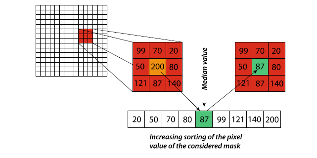
Median Filter
The median filter attenuates the loss of image sharpness and blurring level. It stores every pixel with the value of the median pixel obtained after the pixels of the neighbourhood within window size $L× L$ have been sorted in increasing order. The median pixel has the highest value of the first half of the pixels in neighbourhood, and the lowest value of the other half of the remaining pixels.
In general window dimension of $L× L$, the position of the median pixel is the $(L × L//2+1)-th$
Minimum and Maximum Filter
These filters can collectively called Rank Filtering. The approach here is same as in median filter,, and produce a sorted list in the selected vicinity of $L× L$ window.
The minimum filters introduces an image darkening in the filtered image (moves the histogram of the levels towards the low value). Similarly, the maximum filter tends to lighten the image (moves the histogram of the levels towards the high value).
While, median filter removes the impulsive noise, the minimum filter tends to remove the isolated white dots, and maximum filter tends to remove the isolated black dots.
Gaussian Smoothing Filter
These filters define the coefficient of the Convolution mask according to Gaussian function, and are effective for attenuating Gaussian noise in the image. The impulse response function $h(l,k)$, modeled by the discrete Gaussian fuction with zero mean, is given by :
$\hspace{3em} h(l,k) = c ⋅ e^{-\frac{l^2 + k^2}{2σ^2}}$
where $\sigma$ is the standard deviation of the associated probability distribution, $c$ is the normalization factor which is assumed to be equal to $1$.
The weight of the mask coefficients is inversely proportional to the pixel distance from central one (pixels at a distance greater than $3\sigma$ will have no influence for filtering). Few properties of the Gaussian Filter are :
Circular Symmetry
Gaussian function is the only filter that has the property of Circular symmetry. It is demonstrated by converting the Cartesian coordinates $(l,k)$ into polar coordinates $(r,\theta)$ in the Gaussian fucntion.
$\hspace{3em} h(r,\theta) = c⋅ e^{-\frac{r^2}{2σ^2}}$
where the polar radius $r$ is defined by $r^2 = l^2 + k^2$ The circular symmetry property is demonstrated by the non-dependence of $h(r,\theta)$ from the azimuth $\theta$.