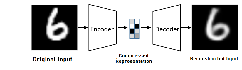
AutoEncoders are a specific kind of neural networks, a bridge between supervised and unsupervised. It first encodes the input into a compressed form and learns from it in an un-supervised manner a meaningful representation that helps to decode it back into a re-constructed input, hopefully as similar as the original input. When it was first introduced, it was used with linear activation function as a technique for dimensionality reduction.
AutoEncoder (AE) Architecture
AE consists of an encoder and decoder, where the encoder is a function $f$ that maps an input $x ∈ \mathbb{R}^d$ to hidden representation $h(x) ∈ \mathbb{R}^d$. The Encoder has the form:
$\hspace{3em} h = f(x) = s_{f}(Wx + b_{h})$
where $s_{f}$ is a non-linear activation function, typically a sigmoid function $(z) = \frac{1}{1+e^{-z}}$. The encoder is parameterized by a $d_{h} × d_{x}$ weight matrix $W$, and a bias vector $b_{h} ∈ \mathbb{R}^d$
Similarly, the decoder function $g$ maps hidden representation $h$ back to a reconstruction $y$
$\hspace{3em} y = g(h) = s_{g}(W’h + b_{y})$
where, $s_{g}$ is the decoder’s activation function, typically either the identity (yielding linear reconstruction) or a sigmoid. The decoder’s parameters are a bias vector $b_{y} ∈ \mathbb{R}^d$, and matrix $W’$.
While training AutoEncoder, we try to find parameters $θ = {W,b_{h},b_{y}}$ that minimizes the reconstruction error on a training set of examples $D_{n}$. Then, our objective function can be written as :
$\hspace{3em} J_{AE}(θ ) = \sum\limits_{x ∈ D_{n}} L(x,g(f(x)))$
where, $L$ is the reconstruction error. Usually, it is $l_{2}$ norm i.e, $L(x,y) = \lVert x-y \rVert^2$ in cases of linear reconstruction, and the cross-entropy loss when $s_{g}$ is the sigmoid. A basic AutoEncoder Architecture can be seen below :
Regularized AutoEncoder
As AutoEncoder are in a way a tool for feature extraction, and therefore, it is always better to have more and more features extracted from the input. If we leave hidden node with less than the size of node in input, it can overfit.
On the other hand, if we add equal or greater number of nodes in the hidden layer than the input node, it will simply the learn and pass the input representation. This is the case, we call - over-complete hidden layer.
Therefore, we need to have some additional regularization added into network, so that more and more feature can be extracted into representation, without being overfit, and underfit. Few key Regularized AutoEncoder are discussed below:
Sparse AutoEncoders
In Sparse AutoEncoder, there are actually two ways to enforce sparsity regularization, where regularization is applied on the activations instead of the weights.
First way to induce sparsity is to apply $L_{1}$ regularization, the autoencoder optimization then becomes :
$\hspace{3em} J_{SparseAE} = \left(\sum\limits_{x ∈ D_{n}}L(x,g(f(x)))\right) + λ \sum\limits_{i} \lvert a_{i} \rvert$
where, $a_{i}$ is the activation at the $i$-th hidden layer and $i$ iterates over all the hiddens activations.
Second way is to use KL-divergence, which is a measure of the distance between two probability distributions. here, we assume the activation of each neuron acts as a Bernoulli variable with probability $p$. Then, at each batch, the actual probability is then measured, and the difference between two $p$ distribution is applied as a regularization factor.
For each neuron $j$ the calculated empirical probability is $p_{j} = \frac{1}{m} \sum\limits_{i} a_{i}(x)$, where $i$ iterates over the samples in the batch. The overall loss function then becomes
$\hspace{3em} J_{SparseAE} = \left(\sum_{x ∈ D_{n}}L(x,g(f(x)))\right) + \sum\limits_{j} KL (p \lVert p’_{j})$
where, the regularization term in it aims at matching \(p\) to \(p^{'}\)