Probability distributions describe how probabilities are distributed over the values of a random variable. They can be broadly classified into two types, i.e, Discrete Probability Distributions and Continuous Probability Distributions. Understanding these two categories is essential before exploring specific distributions like normal, binomial poisson, etc.
Discrete Probability Distribution
A discrete probability distribution is deifned on a set of discrete or countable values, and the probabilities of each value are given by the Probablity Mass Function (PMF) denoted by $P(X = x)$. The PMF specifies the probabilities that the random variable $X$ takes the value $x$. Discrete probability distributions are used to model variables that are distinct, finite and separate such as number of kids in a family
The properties of a discrete probability distribution are :
- The sum of probabilities over all possible values of $X$ is equal to 1 i.e, $\sum P(X = x) = 1$
- The probabilities are non-negatives $P(X = x) \ge 0$ for all $x$
- The probability of each value of $X$ is between 0 and 1 i.e, $0 \le P(X=x)\le1$ for all $x$
Binomial Distribution
Binomial Distribution describes the number of successes in fixed number of independent Bernoulli trails, where each trail has a Boolean-valued outcome: success (with probability $p$) or failure (with probability $q = 1-p$)
The Probability Mass Function (PMF) of Binomial distribution is given by :
\[P(X=k) = \binom{n}{k} p^k (1-p)^{n-k}\]for $k = 0,1,2,…,n$ where
$n$ is number of trails, $p$ is number of successes, $X$ is the random variable that represents the no. of successes in $n$ trials, and $k$ is integer representing number of successes, and $\binom{n}{k}= \frac{n!}{k!(n-k!)}$
The Cumulative Distribution Function (CDF) of Binomial distribution is given by :
\[f(x) = P(X \le x) = \sum_{k=0}^x \binom{n}{k} ⋅ p^k ⋅ (1-p)^{n-k}\]The mean of binomial is $\mu = np$ and the variance of binomial distribution is $\sigma^2 = np(1-p)$. In binomial distribution, as the number of trials n increases, it becomes more symmetrical and approaches a normal distribution.
Negative-Binomial Distribution
It has the same construct as binomial distribution having a series of independent Bernoulli trials, where each trial has a Boolean-valued outcome: success with p probability and failure with $q = 1-p$ probability.
However, Negative-Binomial counts number of trials required to achieve r successes, unlike Binomial that counts successes in a fixed number of trials.
The PMF of the Negative-Binomial Distribution is given by:
\[P(X = k) = \binom{k-1}{r-1}⋅ p^r ⋅ (1-p)^{k-r} \qquad \text{for}\quad k = r, r+1, r+2, \cdots\]where $k$ is total number of trials, $r$ number of successes needed, and $p$ the probability of success in each trial.
Alternatively, it can also expressed in terms of failures $Y$ before the $r$-th success. Here, we have $Y = X-r$ and newer form is given by:
\[P(Y = y) = \binom{r+y-1}{y}⋅ p^r ⋅ (1-p)^y \qquad y=0,1,\cdots\]Mean of $X∼\text{Neg-bin}(r, p)$ is $\frac{r}{p}$ and variance is $\frac{r(1-p)}{p^2}$
Geometric Distribution
It is one of the simplest of waiting time distribution, and special case of Negative-Binomial where $r=1$ i.e, number of trials until the first success.
Here, the PMF of geometric distributio is as:
\[P(X = k) = p(1-p)^{k-1} \qquad k = 1, 2, \cdots\]where, $p$ is probability of success, and $k$ is number of trails. With $r=1$, we have mean of Geometric Distribution as $\frac{1}{p}$, and variance as $\frac{1-p}{p^2}$
Multinomial Distribution
Multinomial distribution is an extension on binomial for cases we have more than two possible outcomes i.e, each trial has $k \ge 2$ possible outcomes. Its PMF can be given by:
\[P(X_{1} = x_{1}, X_{2} = x_{2}, \cdots, X_{k} = x_{k}) = \frac{n!}{x_{1}!⋅ x_{2}!\cdots x_{k}!}p_{1}^{x_{1}}p_{2}^{x_{2}}\cdots p_{k}^{x_{k}}\] \[P(X=x) = \frac{n!}{Π x_k!}Π p_k^{xk}\]where,
$n ∈ {0,1,2,\cdots}$ is total number of trials,
$k\gt 0$ is number of mutually exclusive events, and $x_{i}$ is number of times outcome $i$ occurs
$p_1, p_2, \cdots p_k$ is event probabilities such that $p_1 + p_2 + \cdots p_k =1 \quad \text{i.e,}\sum_{i=1}^k p_{i}=1$
Expected number of times outcomes $i$ occured over $n$ times or Mean is $\mathbb{E}(X_{i}) = np_{i}$, variance $\text{var}(X) = np_{i}(1-p_{i})$ and covariance, $\text{Cov}(X_i, X_j) = -np_{i}p_{j}$
Poisson Distribution
Poisson distribution describes the number of events that occur in a fixed interval of time or space, given the average rate of occurence. It is used to model a wide range of real-world phenomena, such as accident at a busy intersection in a day, and particularly useful for situations where the events are rare or infrequent but can occur at any time.
The PMF of a poisson distribution is given by:
where,
- $k$ is the number of events that occur in the interval.
- $λ$ is the expected number of eventa that occur in the interval.
The Mean and Variance of the poisson distribution are both equal to $\lambda$. The key thing in poisson distribution is that the events are independent of each other, and occur at a constant rate over time and space. In other words, the probability of an event occuring does not depend on when and where the previous event occured. This is known as Poisson Process.
Continuous Probability Distribution
A continuous probability distribution is defined on a continuous range of values, and the probabilites of each value are given by the Probability Density Function (PDF) denoted by $f(x)$.
The PDF specifies the probability density at each point $x$.
The properties of a continuous probability distribution are :
- The total area under the curve of the PDF is equal to 1 i.e, $∫ f(x)dx=1$
- The PDF is non-negative $f(x)\ge0$ for all $x$
- The probability of any particular value is zero. $P(X=x) = 0$ for all $x$.
- The probability of $X$ falling within a range of values is given by the integral of the PDF over that range $P(a\le X\le b) = \int_{a}^b f(x) dx$.
Continuous probability distributions are used to model variables that can take on any value within a range, such as time, and temperature. This is another difference, in discrete distribution, probablities are assigned to each possible outcomes, whereas in continuous distribution, probabilities are assigned to interval of values.
Uniform Distribution
The uniform distribution is a continuous probability distribution where all outcomes in a given range are equally likely. It is defined on an interval closed or open, $[a, b]$ or $(a,b)$ where $a$ is minimum and $b$ is maximum value. PDF is given by:
\[f(x) = \begin{cases} \frac{1}{b - a}, & \text{if } a \le x \le b, \\ 0, & \text{otherwise.} \end{cases}\]Mean, $\mu$ is $\frac{a+b}{2}$ and variance, $\sigma^2 = \frac{(b-a)^2}{12}$. The cumulative distribution function (CDF) of uniform distribution is given by:
\[F(x) = \begin{cases} 0 & \text{for}\quad x \lt a,\\ \frac{x-a}{b-a} & \text{for} \quad a\le x \le b, \\ 1 & \text{for} \quad x \gt b \end{cases}\]Normal Distribution
Normal or Gaussian Distribution is the most commonly used continuous probability distribution in statistics due to the central limit theorem. It is symmetric, bell-shaped and defined over $(-\infty, \infty)$, with mean and mode at $\mu$ and variance $\sigma^2$. Standard normal distribution is special case when $μ =0$ and $\sigma^2 = 1$. It can be denoted as $X∼ \mathcal{N}(0,1)$. The PDF of normal distribution is given by:
\[f(x) = \frac{1}{σ \sqrt{2\pi}}e^{-\frac{(x-\mu)^2}{2\sigma^2}}\]Alternative Parameterization : It uses the term precision $\tau$ instead of standard deviation $\sigma$, where $τ = \frac{1}{\sigma^2}$. This makes numerical computation easier and given as:
\[f(x) = \sqrt{\frac{\tau}{2\pi}}e^{-\tau(x-\mu)^2}/2\]Log-Normal Distribution
The Log-Normal distribution is a distribution of random variable whose logarithm is normally distributed. If $Y = \log(X)$ follows a normal distribution with parameters $\mu$ and $\sigma$, then $X$ follows a log-normal distribution. Its PDF is given by:
\[f(x) = \frac{1}{x\sigma\sqrt{2\pi}}e^{-\frac{(\log x - \mu)^2}{2\sigma^2}}\]Mean and variance of Log-Normal are:
\[μ = e^{μ + \frac{\sigma^2}{2}}\] \[\sigma^2 = (e^{\sigma^2} -1)e^{2μ + \sigma^2}\]The shape of the log-normal distribution is positively skewed. It is often used to model variables that must be positive and have right-skewed distributions, such as income, stock prices, or any growth rate.
Beta Distribution
The beta distribution is a continuous probability distribution that is often used to model the probability of success or failure in a binomial experiment. It is defined on the interval $[0,1]$, and has two parameters $\alpha$ and $\beta$ which control its shape and location. Its PDF is given by:
\[f(x:\alpha, \beta) = x^{\alpha-1}(1-x)^{\beta-1} \frac{1}{(B(\alpha,\beta))}\]where,
- $x$ is the random variable representing the probability of success
- $\alpha$ and $\beta$ are the shape paramters of the distribution
- $B(\alpha, \beta)$ is the beta function, which is used to ensure that the total probability of the distribution to $1$
Mean and variance of the beta distribution are given by :
\[μ = \frac{\alpha}{α + \beta}\] \[\sigma^2 = \frac{(α \cdot \beta)}{[(α + \beta)^2 \cdot (α + β + 1)]}\]The shape of the beta distribution depends on the values of the shape parameters $\alpha$ and $\beta$. When $α = β = 0$, the distribution is uniform distribution, with equal probability assigned to all values between 0 and $1$. When $α \ge \beta$, the distribution is skewed towards the right, with a mode close to $1$. When $α \le \beta$, the distribution is skewed towards the left with a mode close to 0.
Exponential Distribution
It is a continuous probability distribution that decribes the time between two consecutive events in a Poisson Process. The Exponential distribution is mostly used to model the lifetime of a product or the time until a failure occurs in a system.
The probability density function (PDF) of exponential distribution is given by :
\[f(x) = λ e^{-λ x} \quad \text{for}\; x \ge 0\] \[f(x) = 0 \qquad \text{for}\; x \lt 0\]where, $\lambda$ is rate paramter i.e, average number of events occuring per unit of time, and $x$ is time elapsed since last event.
The Cumulative Distribution Function (CDF) of exponential is given by :
\[f(x) = 1 - e^{-λ x} \quad \text{for}\; x \ge 0\] \[f(x) = 0 \qquad \text{for}\; x \lt 0\]Alternative Parameterization
Exponential distribution, sometimes, can parameterized in terms of the scale parameter $\beta = \frac{1}{\lambda}$,then:
\[\text{PDF:} \quad f(x) = \frac{1}{\beta} ⋅ e^{\frac{-x}{\beta}}\quad \text{for}\; x \ge 0\] \[\quad f(x) = 0 \qquad \text{for}\; x \lt 0\] \[\text{CDF:} \quad f(x) = 1 - e^{\frac{-x}{\beta}} \quad \text{for}\; x \ge 0\] \[\quad f(x) = 0\qquad \text{for}\; x \lt 0\]The mean and variance of Exponential Distribution are: $\mu = \frac{1}{\lambda}$ and $\sigma^2 = \frac{1}{\lambda^2}$, respectively.
Gamma Distribution
It is a continuous probability distribution, mostly used to model the sum of independent exponentially distributed random variables. The Gamma Distribution is defined by two parameters: $\alpha$ shape parameter and $\beta$ rate parameter.
The Probability Density Function (PDF) of Gamma Distribution is given by:
\[f(x; \alpha, \beta) = \frac{\beta^\alpha}{\Gamma(\alpha)}x^{α - 1}e^{-β x} \quad \text{for}\; x \gt 0 \quad \; \alpha, β \gt 0\]where, $x$ is a non-negative real number, $Γ(α)$ is the gamma function, and $\alpha$ and $\beta$ are the shape and rate parameters, respectively. The PDF is defined for $x \ge 0$.
The Gamma Function is defined as:
$\Gamma(a) = \int_{0}^{\infty} t^{α - 1} e^{-t}\,dt$ For all positive integers, $\Gamma(\alpha) = (α - 1)!$
The cumulative distribution function (CDF) of the Gamma distribution is given by:
\[F(x; α, β) = \frac{1}{Γ(α)} \cdot γ(α, βx)\]where, $γ(α, βx)$ is the lower incomplete gamma function, defined as: $γ(α, βx) = \int_{0}^x t^{α - 1} e^{-β t} dt$
The Mean of Gamma Distribution is: $μ = \frac{\alpha}{\beta}$ and variance is: $\sigma^2 = \frac{\alpha}{\beta^2}$.
The shape parameter $\alpha$ determines the shape of the distribution, while the rate parameter $β$ determines the rate at which the distribution decays. As $α$ increases, the Gamma distribution becomes more peaked and skewed to the right, while as $β$ increases, the distribution becomes more concentrated around the mean.
Inverse-Gamma Distribution
The inverse-gamma distribution is a two-parameter family of continuous distribution over $x \gt 0$. It is mainly used as a prior for variance parameter in bayesian statistics. It has two parameters: shape parameter, $\alpha$, and scale parameter, $\beta$ unlike Gamma distribution where $β$ is rate parameter.
PDF of Inverse-Gamma is given as:
\[f(x) = \frac{\beta^{\alpha}}{\Gamma(\alpha)}x^{-\alpha-1}e^{-\frac{\beta}{x}}\]Similarly, the CDF of Inverse-Gamma distribution can be given as:
\[F(x) = \frac{Γ \left(\alpha, \frac{\beta}{x}\right)}{\Gamma(\alpha)} = Q\left(\alpha, \frac{\beta}{x}\right)\]where, numerator is incomplete gamma function, denominator is gamma function and Q is regularized gamma function
Mean and variance of inverse-gamma are as follows:
\[μ = \frac{\beta}{α -1}, \qquad α \gt 1\] \[\sigma^2 = \frac{\beta^2}{(\alpha-1)^2(\alpha-2)}, \qquad α \gt 2\]Weibull Distribution
The Weibull Distribution is a continuous distribution commonly used to model a broad range of random variable for time-to-failure ot time between events. It is defined over $x\ge 0$ and has two paramters: the shape $k$ and the scale $λ$. Its PDF is given by:
\[f(x) = \begin{cases} \frac{k}{\lambda} \left(\frac{x}{\lambda}\right)^{k-1} e^{-\left(\frac{x}{\lambda}\right)^k}, & x \geq 0, \\ 0, & \text{otherwise.} \end{cases}\]where,x is the random variable representing time-to-failure, $k\gt 0$ is the shape parameter, and $λ \gt 0$ is the scale parameter.
- A value of $k \lt 1$ indicates that failure rate is decreasing over time
- A value of $k = 1$ indicates that the failure rate is constant over time. It reduces Weibull distribution to exponential distribution
- A value of $k \gt 1$ indicates that the failure rate increasing over time.
Mean and variance of Weibull distribution are as follows:
\[μ = λΓ\left(1+\frac{1}{k}\right)\] \[\sigma^2 = \lambda^2 \left[ \Gamma\left(1 + \frac{2}{k}\right) - \left(\Gamma\left(1 + \frac{1}{k}\right)\right)^2 \right]\]The CDF for Weibull Distribution is as:
\[F(x) = \begin{cases} 1 - e^{-(\frac{x}{\lambda})^k} & x \ge 0 \\ 0, & \text{otherwise} \end{cases}\]If $x = \lambda$, then, $F(x) = 1 -e^{-1} ≈ 0.632$
Dirichlet Distribution
Dirichlet $\text{Dir}(\alpha)$ or multivariate beta distribution (MBD) is a multivariate generalization of beta distribution paramterized by a vector $\alpha$ of positive reals. It is commonly used as prior in bayesian stat, and conjugate prior of multinomial distribution.
It is defined on the $(K-1)-$dimensional simplex, where each column vector $x = (x_{1}, x_{2}, \cdots, x_{k})$ satisfies $x_{i}\ge 0$ and $\sum_{i=1}^K x_{i}=1$. Its PDF is given as:
\[f(x) = \frac{1}{\mathcal{B}(\alpha)}\Pi_{i=1}^K x_{i}^{\alpha_{i}-1}\]where,
- $α = (\alpha_{1}, \alpha_{2}, \cdots, \alpha_{k})$ are concentration parameters, $\alpha_{i} \gt 0$ and $\mathcal{B}(\alpha) = \frac{\Pi_{i=1}^K \Gamma(\alpha_{i})}{\Gamma(\sum_{i=1}^K \alpha_{i})}$
Mean and variance for each component are as follows:
\[\mathbb{E}[X_{i}] = \frac{\alpha_{i}}{\alpha_{0}}, \qquad \text{where} \alpha_{0} = \sum_{i=1}^K \alpha_{i}\] \[\text{Var}[X_{i}] = \frac{\alpha_{i}(\alpha_0 - \alpha_i)}{\alpha_{0}^2(\alpha_{0}+1)}\]Logistic Distribution
Logistic Distribution is a continous distribution used for modelling growth, and it resembles the normal distribution but has higher kurtosis. The PDF of logistic distribution can be given as:
\[f(x) = \frac{e^{-(x-μ)/s}}{s(1+e^{-(x-\mu)/s})^2}\]where,
$x$ is random variable, $\mu$ is the location parameter, and $s \gt 0$ is the scale parameter.
Its CDF is logistic function which is used in logistic regression and neural networks. It is given below:
\[F(x) = \frac{1}{1+e^{-(x-\mu)s}}\]Mean, median and mode of logistic distribution have same value of $\mu$, and variance is $\frac{s^2\pi^2}{3}$
Degree of Freedom
Degree of freedom (df) is the number of independent observations or sample values that go into estimating a parameter or testing a hypothesis.
Mathematically, the degree of freedom (df) is defined as the number of values in a sample that are free to vary after certain restrictions have been imposed. For example, if we have a sample of size $n$, and we know the sample mean, then there are $n-1$ degrees of freedom remaining because we can calculate any $n-1$ values in the sample and the mean constraint will tell the $n^{th}$ value.
Chi-Squared Distribution
It is continuous probability distribution widely used in hypothesis testing and goodness-of-fit observation. It has just one parameter: a positive integer $k$ specifying degree of freedom.
If $Z_1, …, Z_k$ are independent standard normal randon variable, then sum of their squares i.e, $Q = \sum_{i=1}^k Z_i^2$ is distributed according chi-squared distribution with $k$ degree of freedom, usually denoted as $Q ~ X^2(k)$ This is why Chi-Squared distribution is used because in the cases of hypothesis testing when the sample size $n$ increases, the sampling distribution start to approach normal distribution.
Therefore, in machine learning, the chi-squared test can be used to evaluate the relevance of a feature by calculating the dependence between the feature and the target variable. Features with a high chi-squared value are considered to be more relevant, and can be selected for further analysis.
Similarly, it can be used in model evaluation - to test whether the difference between the observed and expected values is statistically significant.
The probability density function (PDF) of Chi-Squared is given as:
\[f(x;k) = \frac{x^{\frac{k}{2} -1}e^{-\frac{x}{2}}}{2^{\frac{k}{2}} ⋅ \Gamma(\frac{k}{2})} \quad \text{for}\; x\gt 0\]and PDF is $0$ otherwise.
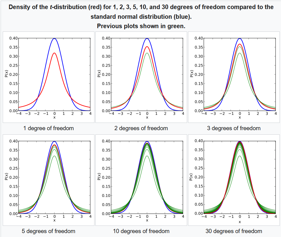
Student’s t-distribution
It is another continuous probability distribution. It arises in statistics, when the mean of a normally distributed population in situations where the sample size is small and the populations standard deviation is unknown. It is used in assessing statistical significance, and creating confidence interval.
If we take a random sample of $n$ observations from a normal distribution, then the t-distribution with $ν = n - 1$ degrees of freedom can be defined as the distribution of the location of the sample mean in relation to the true mean, divided by the sample standard deviation, and then multiplied by the standardizing factor of $\sqrt{n}$.
Using the t-distribution, then, allows us to create a confidence interval for the true mean.
The Probability Density Function (PDF) of the Student’s t-distribution with $v$ degree of freedom is given by:
$\begin{equation} \Large f(x;v) =\frac{Γ(\frac{v+1}{2})}{\sqrt{v}\pi Γ(\frac{v}{2})} (1 + \frac{t^2}{v})^{-\frac{v+1}{2}}\end{equation}$
Key things on student’s t-distribution:
- Its PDF is symmetric around zero.
- Its overall shape resembles the bell shape of a normally distributed variable with mean 0 and variance 1, except that it is a bit lower and wider.
- As the number of degrees of freedom grows, the t-distribution approaches the normal distribution with mean $0$ and variance $1$. For this reason $v$ is also known as the normality parameter.
F-Distribution
F-Distribution is another continuous probability function, used in analysis of variance (ANOVA) and other F-tests. It is a ratio of two chi-squared distribution with degree of freedom as parameter given below:
$X = \frac{U_1/d_1}{U_2/d_2}$
where $U_1$, and $U_2$ are chi-squared distributions with $d_1$ and $d_2$ as their degree of freedom, respectively. Also, similar to student t-distribution as degree to freedom start to increase, distribution starts to look like normal distribution.
The probability density function (PDF) of f-distribution is given by:
$\begin{equation} \Large f(x;d_1, d_2) = \frac{\sqrt{\frac{(d_1x)^{d_1} d_2^{d_2}}{(d_1x +d_2)^{d_1+d_2}}}}{xB(\frac{d_1}{2}, \frac{d_2}{2})} \end{equation}$